

Two-Sample Inference on the Circle#
Two samples of manifold-valued observations can differ in location, spread, or their complete empirical distributions. GeoJAX exposes several tests with different sensitivities:
Fréchet ANOVA compares group means and Fréchet variances;
the Biswas–Ghosh test combines within- and between-group distances; and
energy distance compares cross-sample and within-sample distances;
maximum mean discrepancy compares empirical kernel embeddings; and
the Wasserstein test compares the two weighted empirical measures through an exact transport problem.
These are not interchangeable p-values for one universal null statistic. They encode distinct summaries of the same metric data [Biswas and Ghosh, 2014, Dubey and Müller, 2019, Gretton et al., 2012, Székely and Rizzo, 2013].
from pathlib import Path

import jax
jax.config.update("jax_enable_x64", True)
import jax.numpy as jnp
import matplotlib.pyplot as plt
import numpy as np

from geojax.geometry import Sphere
from geojax.learning import (
    biswas_ghosh_two_sample_test,
    energy_two_sample_test,
    frechet_anova,
    kernel_mmd_two_sample_test,
    pairwise_distances,
    wasserstein_two_sample_test,
)

plt.rcParams.update({
    "figure.dpi": 220,
    "savefig.dpi": 320,
    "font.size": 10,
    "axes.titlesize": 11,
    "axes.spines.top": False,
    "axes.spines.right": False,
})

M = Sphere(size=2)
key_x, key_y = jax.random.split(jax.random.key(270))
angles_x = -0.48 + 0.22 * jax.random.normal(key_x, (9,))
angles_y = 0.38 + 0.27 * jax.random.normal(key_y, (9,))

def on_circle(angles):
    return jnp.stack([jnp.cos(angles), jnp.sin(angles)], axis=-1)

x = on_circle(angles_x)
y = on_circle(angles_y)
pooled = jnp.concatenate([x, y], axis=0)
groups = jnp.concatenate([
    jnp.zeros(len(x), dtype=int),
    jnp.ones(len(y), dtype=int),
])

fanova = frechet_anova(M, pooled, groups, method="asymptotic")
distance_test = biswas_ghosh_two_sample_test(
    M, x, y, n_permutations=99, key=jax.random.key(271)
)
energy_test = energy_two_sample_test(
    M, x, y, n_permutations=99, key=jax.random.key(273)
)
# cos(d(x, y)) is the ambient inner-product kernel on the unit circle.
mmd_test = kernel_mmd_two_sample_test(
    M,
    x,
    y,
    kernel=lambda distances: jnp.cos(distances),
    n_permutations=99,
    key=jax.random.key(274),
)
transport_test = wasserstein_two_sample_test(
    M, x, y, p=2.0, n_permutations=19, key=jax.random.key(272)
)

print(f"{'test':24s} {'statistic':>11s} {'p-value':>10s}")
print("-" * 48)
for name, result in (
    ("Fréchet ANOVA", fanova),
    ("Biswas-Ghosh", distance_test),
    ("Energy distance", energy_test),
    ("Kernel MMD", mmd_test),
    ("Wasserstein", transport_test),
):
    print(f"{name:24s} {float(result.statistic):11.5f} {float(result.pvalue):10.4f}")
test                       statistic    p-value
------------------------------------------------
Fréchet ANOVA              124.44356     0.0000
Biswas-Ghosh                 0.33964     0.0100
Energy distance              0.86783     0.0100
Kernel MMD                   0.42540     0.0100
Wasserstein                  0.70228     0.0500
Permutation p-values are computed with the finite-sample correction
Consequently, the smallest possible values in this tutorial are \(1/100\) for the distance, energy, and MMD tests and \(1/20\) for Wasserstein. The transport count is intentionally small because every permutation solves an exact linear transport problem. Substantially more permutations are required for a final analysis; these counts keep the executable demonstration quick and deterministic. Their finite-sample interpretation requires exchangeability of the pooled labels under the null. Moreover, energy and related distance statistics characterize equality in distribution only under appropriate metric-space conditions, such as strong negative type; the permutation calculation alone does not establish that geometric property.
Visual report#
The distance matrix displays the block structure seen by the metric tests. Four panels place observed statistics against their permutation null distributions. Fréchet ANOVA uses its documented asymptotic reference law and is reported numerically above.
distances = pairwise_distances(M, pooled)

fig, axes = plt.subplots(2, 3, figsize=(13.4, 7.2), constrained_layout=True)
axes = axes.ravel()
circle = np.linspace(-np.pi, np.pi, 500)
axes[0].plot(np.cos(circle), np.sin(circle), color="0.80", linewidth=1.1)
axes[0].scatter(
    np.asarray(x[:, 0]), np.asarray(x[:, 1]),
    color="#2563EB", s=34, edgecolor="white", linewidth=0.35, label="sample X",
)
axes[0].scatter(
    np.asarray(y[:, 0]), np.asarray(y[:, 1]),
    color="#E45756", marker="s", s=34, edgecolor="white", linewidth=0.35,
    label="sample Y",
)
axes[0].set(aspect="equal", xlim=(-1.1, 1.1), ylim=(-1.1, 1.1), title="Observed samples")
axes[0].set_xticks([])
axes[0].set_yticks([])
axes[0].legend(frameon=False, loc="center")

image = axes[1].imshow(np.asarray(distances), cmap="magma", origin="lower")
axes[1].axhline(len(x) - 0.5, color="white", linewidth=0.8)
axes[1].axvline(len(x) - 0.5, color="white", linewidth=0.8)
axes[1].set(title="Geodesic distance matrix", xlabel="observation", ylabel="observation")
fig.colorbar(image, ax=axes[1], shrink=0.78)

for axis, result, title, color in (
    (axes[2], distance_test, "Biswas--Ghosh null", "#009E8E"),
    (axes[3], energy_test, "Energy-distance null", "#2563EB"),
    (axes[4], mmd_test, "Kernel-MMD null", "#E45756"),
    (axes[5], transport_test, "Wasserstein null", "#7C3AED"),
):
    null = np.asarray(result.null_distribution)
    axis.hist(null, bins=16, color=color, alpha=0.72, edgecolor="white")
    axis.axvline(
        float(result.statistic), color="#111827", linestyle="--", linewidth=2.0,
        label=f"observed\n$p={float(result.pvalue):.3f}$",
    )
    axis.set(title=title, xlabel="permuted statistic", ylabel="count")
    axis.legend(frameon=False)
    axis.grid(axis="y", alpha=0.18)

output = next(
    path for path in (
        Path("../_static/tutorials/two-sample-inference.png"),
        Path("docs/_static/tutorials/two-sample-inference.png"),
        Path("_static/tutorials/two-sample-inference.png"),
    )
    if path.parent.exists()
)
output.parent.mkdir(parents=True, exist_ok=True)
fig.savefig(output, bbox_inches="tight")
plt.show()
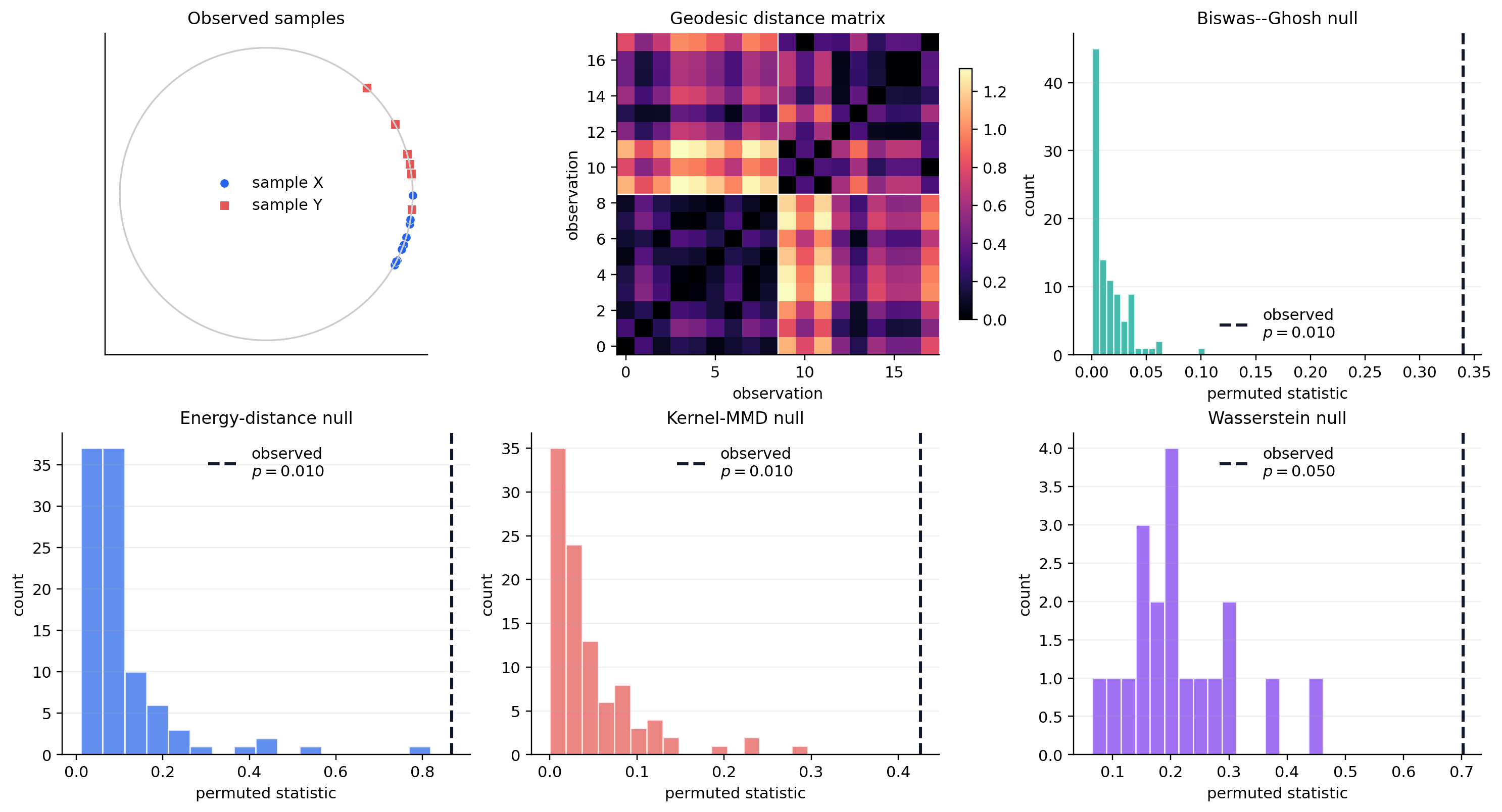
A significant result identifies evidence against the corresponding equality hypothesis; it does not establish which geometric feature generated the difference. The plots, effect sizes, group summaries, and study design remain part of the analysis.
References#
Munmun Biswas and Anil K. Ghosh. A nonparametric two-sample test applicable to high dimensional data. Journal of Multivariate Analysis, 123:160–171, 2014. doi:10.1016/j.jmva.2013.09.004.
Paromita Dubey and Hans-Georg Müller. Fréchet analysis of variance for random objects. Biometrika, 106(4):803–821, 2019. doi:10.1093/biomet/asz052.
Arthur Gretton, Karsten M. Borgwardt, Malte J. Rasch, Bernhard Schölkopf, and Alexander Smola. A kernel two-sample test. Journal of Machine Learning Research, 13(25):723–773, 2012. URL: https://www.jmlr.org/papers/v13/gretton12a.html.
Gábor J. Székely and Maria L. Rizzo. Energy statistics: a class of statistics based on distances. Journal of Statistical Planning and Inference, 143(8):1249–1272, 2013. doi:10.1016/j.jspi.2013.03.018.