

Intrinsic k-means in the hyperbolic plane#
Euclidean k-means alternates nearest-center assignments and arithmetic means [Lloyd, 1982]. On a Riemannian manifold, distances become geodesic and each center becomes a Frechet mean [Fréchet, 1948, Karcher, 1977]. For clusters \(G_1,\ldots,G_K\) on a geometry \(M\), the objective is
Here \(M=\mathbb H^2\) is represented by the upper hyperboloid
The Poincare disk gives a compact view of the same points, while GeoJAX keeps all fitting operations on the hyperboloid. These two equivalent models and their distance geometry are reviewed by Ratcliffe [2006].
from pathlib import Path

import jax
jax.config.update("jax_enable_x64", True)
import jax.numpy as jnp
import matplotlib.pyplot as plt
import numpy as np

from geojax.geometry import Hyperboloid
from geojax.learning import kmeans

plt.rcParams.update({
    "figure.dpi": 220,
    "savefig.dpi": 320,
    "font.size": 10,
    "axes.titlesize": 11,
    "axes.spines.top": False,
    "axes.spines.right": False,
})

M = Hyperboloid(size=3)
disk_centers = jnp.array([
    [-0.52, -0.08],
    [0.32, 0.46],
    [0.43, -0.40],
])
cluster_scales = jnp.array([0.070, 0.065, 0.075])
keys = jax.random.split(jax.random.key(17), 3)

disk_points = jnp.concatenate([
    center + scale * jax.random.normal(key, shape=(18, 2))
    for center, scale, key in zip(disk_centers, cluster_scales, keys)
])
radius = jnp.linalg.norm(disk_points, axis=1, keepdims=True)
disk_points = jnp.where(radius < 0.88, disk_points, 0.88 * disk_points / radius)
points = M.from_poincare(disk_points)

print("number of observations:", points.shape[0])
print("all points lie on H^2:", bool(jnp.all(M.belongs(points))))
number of observations: 54
all points lie on H^2: True
The Gaussian perturbations above are only a convenient way to create a visible synthetic dataset in disk coordinates. They are not presented as an intrinsic probability model. After conversion, every distance, logarithm, exponential, and center update uses the Lorentz geometry.
Lloyd updates through the learning API#
For a nonempty cluster \(G\), a center update averages logarithm vectors in the current tangent space and returns with the exponential map:
This fixed-point calculation is nested inside each Lloyd iteration.
The executable example uses 54 well-separated observations, one seeded
initialization, and a moderate stopping tolerance so the live documentation
build stays quick. For a final scientific fit, increase n_init and
center_maxiter and tighten tol after checking the reported diagnostics.
result = kmeans(
    M,
    points,
    n_clusters=3,
    key=jax.random.key(29),
    init="kmeans++",
    n_init=1,
    maxiter=8,
    center_maxiter=20,
    tol=1e-2,
)

center_disk = M.to_poincare(result.centers)
objective_history = np.asarray(result.diagnostics["objective_history"])

print("estimated centers in the Poincare disk:")
print(np.round(np.asarray(center_disk), 3))
print("cluster sizes:", np.bincount(np.asarray(result.labels)))
print("final mean squared distance:", float(result.objective))
print("termination:", result.reason)
estimated centers in the Poincare disk:
[[ 0.431 -0.409]
 [-0.51  -0.103]
 [ 0.296  0.482]]
cluster sizes: [18 18 18]
final mean squared distance: 0.0961343603354514
termination: objective tolerance reached
Visual report#
The disk boundary is infinitely far away in the hyperbolic metric. The first two panels are therefore model coordinates, not a Euclidean replacement for the fitted geometry. Stars mark the fitted hyperbolic Frechet centers.
palette = np.array(["#E45756", "#009E8E", "#7C3AED"])
boundary = np.linspace(0.0, 2.0 * np.pi, 600)


def setup_disk(axis, title):
    axis.fill(
        np.cos(boundary), np.sin(boundary),
        facecolor="#F8FAFC", edgecolor="#334155", linewidth=1.25,
    )
    axis.set(
        aspect="equal",
        xlim=(-1.04, 1.04),
        ylim=(-1.04, 1.04),
        xlabel="$p_1$",
        ylabel="$p_2$",
        title=title,
    )


fig, axes = plt.subplots(1, 3, figsize=(12.4, 3.8), constrained_layout=True)

setup_disk(axes[0], "Unlabelled disk coordinates")
axes[0].scatter(
    np.asarray(disk_points[:, 0]), np.asarray(disk_points[:, 1]),
    s=22, color="#64748B", alpha=0.72, edgecolor="white", linewidth=0.25,
)

setup_disk(axes[1], "Intrinsic hyperbolic k-means")
labels = np.asarray(result.labels)
for cluster, color in enumerate(palette):
    selected = labels == cluster
    axes[1].scatter(
        np.asarray(disk_points[selected, 0]),
        np.asarray(disk_points[selected, 1]),
        s=23, color=color, alpha=0.78, edgecolor="white", linewidth=0.25,
        label=f"cluster {cluster + 1}",
    )
axes[1].scatter(
    np.asarray(center_disk[:, 0]), np.asarray(center_disk[:, 1]),
    marker="*", s=210, color="#111827", edgecolor="white", linewidth=0.7,
    zorder=5,
)
axes[1].legend(frameon=False, fontsize=8, loc="upper left")

axes[2].plot(
    np.arange(1, objective_history.size + 1), objective_history,
    marker="o", color="#007C83", linewidth=2,
)
axes[2].set(
    title="Lloyd objective",
    xlabel="iteration",
    ylabel="mean squared hyperbolic distance",
)
axes[2].grid(alpha=0.22)

output = next(
    path for path in (
        Path("../_static/tutorials/hyperbolic-kmeans.png"),
        Path("docs/_static/tutorials/hyperbolic-kmeans.png"),
        Path("_static/tutorials/hyperbolic-kmeans.png"),
    )
    if path.parent.exists()
)
output.parent.mkdir(parents=True, exist_ok=True)
fig.savefig(output, bbox_inches="tight")
plt.show()
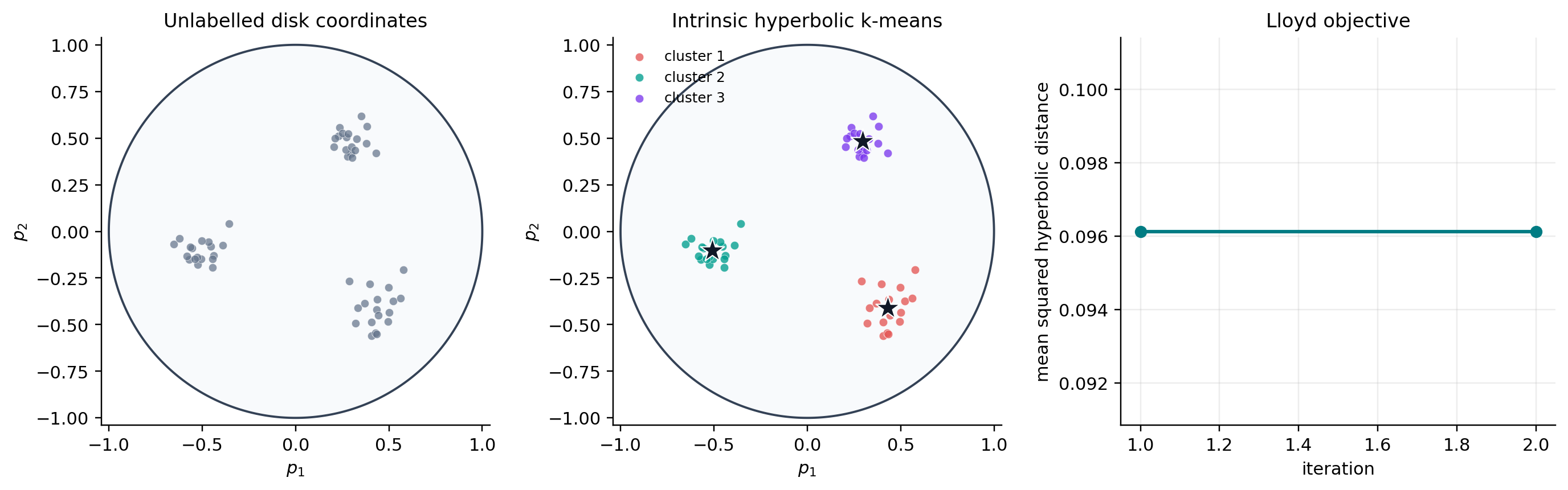
The fitted centers remain on the upper sheet by construction. More importantly, a cluster near the disk boundary is not summarized by an arithmetic average of its displayed coordinates: its center is determined by hyperbolic distances on \(\mathbb H^2\).
What to try next#
Move one group closer to the disk boundary and compare visual and intrinsic spread.
Replace
kmeanswithkmedoidsto restrict representatives to observations.Increase
sizeto cluster points in higher-dimensional hyperbolic space.
References#
Maurice Fréchet. Les éléments aléatoires de nature quelconque dans un espace distancié. Annales de l'Institut Henri Poincaré, 10(4):215–310, 1948. URL: https://www.numdam.org/item/AIHP_1948__10_4_215_0/.
Hermann Karcher. Riemannian center of mass and mollifier smoothing. Communications on Pure and Applied Mathematics, 30(5):509–541, 1977. doi:10.1002/cpa.3160300502.
Stuart P. Lloyd. Least squares quantization in PCM. IEEE Transactions on Information Theory, 28(2):129–137, 1982. doi:10.1109/TIT.1982.1056489.
John G. Ratcliffe. Foundations of Hyperbolic Manifolds. Springer, 2 edition, 2006. doi:10.1007/978-0-387-47322-2.