

Barycentric dictionary learning for covariance matrices#
A Euclidean dictionary reconstructs data by linear combinations of atoms. Positive-definite covariance matrices do not form a vector space under those operations. Intrinsic barycentric coding instead asks for simplex weights \(w\in\Delta^{m-1}\) that approximately satisfy the Karcher equation at an observation \(P\):
We use the log-Euclidean geometry of Arsigny et al. [2007], for which
GeoJAX minimizes the squared Karcher residual plus an \(\ell_2\) ridge term and alternates code estimation with Product-manifold atom optimization [Ho et al., 2013]. The atoms therefore remain SPD matrices throughout learning.
from pathlib import Path

import jax
jax.config.update("jax_enable_x64", True)
import jax.numpy as jnp
import matplotlib.pyplot as plt
import numpy as np

from geojax.geometry import SPDLogEuclidean
from geojax.learning import (
    geodesic_barycentric_coding,
    manifold_dictionary_learning,
)

plt.rcParams.update({
    "figure.dpi": 220,
    "savefig.dpi": 320,
    "font.size": 10,
    "axes.titlesize": 11,
    "axes.spines.top": False,
    "axes.spines.right": False,
})

M = SPDLogEuclidean(size=(2, 2))
latent = jnp.linspace(-1.2, 1.2, 7)


def log_covariance(t):
    return jnp.array([
        [0.48 * t, 0.34 * jnp.sin(1.45 * t)],
        [0.34 * jnp.sin(1.45 * t), -0.24 * t + 0.13 * jnp.cos(1.1 * t)],
    ])


data = jax.vmap(M.expm)(jax.vmap(log_covariance)(latent))
initial_positions = jnp.array([-0.72, 0.03, 0.72])
initial_atoms = jax.vmap(M.expm)(
    jax.vmap(log_covariance)(initial_positions)
)

print("data shape:", data.shape)
print("all observations are SPD:", bool(jnp.all(M.belongs(data))))
data shape: (7, 2, 2)
all observations are SPD: True
The curve is nonlinear in matrix-log coordinates, so three fixed atoms do not reconstruct every observation exactly. A ridge of \(0.1\) makes the simplex code unique and numerically well conditioned; these are dense barycentric codes, not lasso-sparse codes.
initial_codes = geodesic_barycentric_coding(
    M,
    data,
    initial_atoms,
    ridge=0.1,
    maxiter=80,
    tol=1e-5,
    reconstruction_maxiter=5,
)
learned = manifold_dictionary_learning(
    M,
    data,
    n_atoms=3,
    initial_atoms=initial_atoms,
    ridge=0.1,
    maxiter=1,
    coding_maxiter=80,
    center_maxiter=4,
    tol=2e-4,
)

print(f"initial coding objective: {float(initial_codes.objective):.7f}")
print(f"learned dictionary objective: {float(learned.objective):.7f}")
print("simplex sums:", np.round(np.asarray(jnp.sum(learned.codes, axis=1)), 7))
print("outer dictionary updates:", learned.iterations)
initial coding objective: 0.0948966
learned dictionary objective: 0.0577330
simplex sums: [1. 1. 1. 1. 1. 1. 1.]
outer dictionary updates: 1
One outer update keeps this executable documentation compact while still
performing a genuine manifold atom optimization. For a scientific fit, raise
maxiter and monitor diagnostics["objective_history"] until the requested
tolerance is reached.
Visual report#
Each ellipse is a contour of the associated \(2\times2\) covariance matrix. The top and bottom rows compare the initial and learned atoms; the observations occupy the middle row. The second panel shows how barycentric weight moves between atoms along the covariance trajectory.
initial_errors = M.dist(initial_codes.reconstructions, data)
learned_errors = M.dist(learned.reconstructions, data)


def draw_covariance(axis, covariance, center, color, scale, linewidth=1.6, alpha=1.0):
    eigenvalues, eigenvectors = np.linalg.eigh(np.asarray(covariance))
    angle = np.linspace(0.0, 2.0 * np.pi, 180)
    unit_circle = np.vstack([np.cos(angle), np.sin(angle)])
    offsets = eigenvectors @ (np.sqrt(eigenvalues)[:, None] * unit_circle)
    curve = np.asarray(center)[:, None] + scale * offsets
    axis.plot(curve[0], curve[1], color=color, linewidth=linewidth, alpha=alpha)


fig, axes = plt.subplots(1, 3, figsize=(13.5, 4.2), constrained_layout=True)
color_map = plt.get_cmap("viridis")

for index, covariance in enumerate(np.asarray(data)):
    color = color_map(index / (len(data) - 1))
    draw_covariance(
        axes[0], covariance, (float(latent[index]), 0.0),
        color, scale=0.16, linewidth=1.25,
    )
for index, covariance in enumerate(np.asarray(initial_atoms)):
    draw_covariance(
        axes[0], covariance, (float(initial_positions[index]), 1.0),
        "#E45756", scale=0.21, linewidth=1.8,
    )

learned_logs = np.asarray(jax.vmap(M.logm)(learned.atoms))
learned_order = np.argsort(learned_logs[:, 0, 0])
learned_positions = np.array([-0.78, 0.0, 0.78])
for position, atom_index in zip(learned_positions, learned_order):
    draw_covariance(
        axes[0], np.asarray(learned.atoms[atom_index]), (position, -1.0),
        "#009E8E", scale=0.21, linewidth=2.0,
    )
axes[0].set(
    title="Covariance observations and atoms",
    xlim=(-1.55, 1.55),
    ylim=(-1.48, 1.48),
    xlabel="trajectory position",
    yticks=[-1.0, 0.0, 1.0],
    yticklabels=["learned", "data", "initial"],
)
axes[0].grid(axis="x", alpha=0.15)

image = axes[1].imshow(
    np.asarray(learned.codes).T,
    aspect="auto",
    origin="lower",
    cmap="magma",
    interpolation="nearest",
    extent=(float(latent[0]), float(latent[-1]), -0.5, 2.5),
)
axes[1].set(
    title="Barycentric code matrix",
    xlabel="trajectory position",
    ylabel="atom",
    yticks=[0, 1, 2],
)
fig.colorbar(image, ax=axes[1], shrink=0.78, label="weight")

axes[2].plot(
    np.asarray(latent), np.asarray(initial_errors),
    color="#E45756", linestyle="--", marker="o",
    linewidth=1.7, label="initial dictionary",
)
axes[2].plot(
    np.asarray(latent), np.asarray(learned_errors),
    color="#009E8E", marker="o", linewidth=2.0,
    label="learned dictionary",
)
axes[2].set(
    title="Log-Euclidean reconstruction errors",
    xlabel="trajectory position",
    ylabel="distance",
)
axes[2].grid(alpha=0.18)
axes[2].legend(frameon=False, fontsize=8, loc="upper left")

output = next(
    path for path in (
        Path("../_static/tutorials/barycentric-dictionary.png"),
        Path("docs/_static/tutorials/barycentric-dictionary.png"),
        Path("_static/tutorials/barycentric-dictionary.png"),
    )
    if path.parent.exists()
)
output.parent.mkdir(parents=True, exist_ok=True)
fig.savefig(output, bbox_inches="tight")
plt.show()
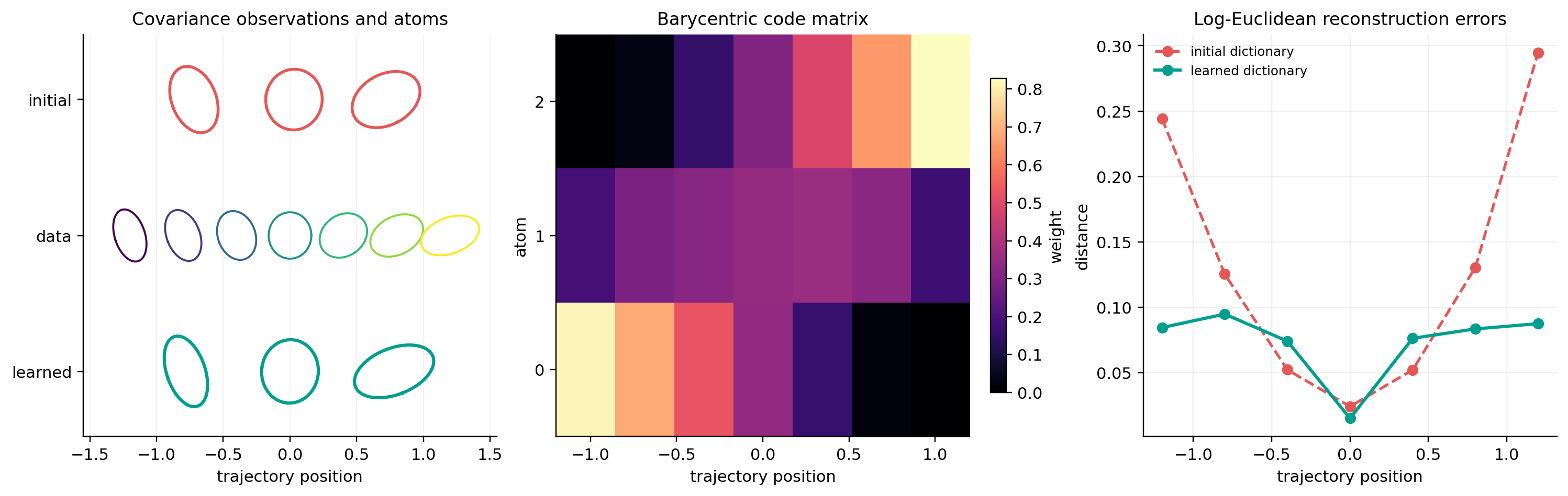
The Karcher equation is local to each observation and depends on the selected geometry. Under the log-Euclidean metric it has a global linearizing chart; under other SPD metrics the same public learning routine uses their own logarithms, exponentials, and inner products instead.
References#
Vincent Arsigny, Pierre Fillard, Xavier Pennec, and Nicholas Ayache. Geometric means in a novel vector space structure on symmetric positive-definite matrices. SIAM Journal on Matrix Analysis and Applications, 29(1):328–347, 2007. doi:10.1137/050637996.
Jeffrey Ho, Yuchen Xie, and Baba Vemuri. On a nonlinear generalization of sparse coding and dictionary learning. In Proceedings of the 30th International Conference on Machine Learning, volume 28 of Proceedings of Machine Learning Research, 1480–1488. 2013. URL: https://proceedings.mlr.press/v28/ho13a.html.