PGA and Regression with SPD Predictors#

Covariance matrices are manifold-valued observations: an arithmetic perturbation can leave the positive-definite cone, while a geometric perturbation remains a valid covariance. Here we generate a one-dimensional covariance trajectory, recover its dominant intrinsic direction with principal geodesic analysis (PGA), and regress a scalar response directly on SPD predictors.

PGA applies ordinary PCA to logarithm vectors at a Fréchet mean, but its Gram matrix is formed with the manifold metric rather than an ambient dot product [Fletcher et al., 2004]. With the log-Euclidean metric,

\[ d(P,Q)=\lVert\log P-\log Q\rVert_F, \]

so this experiment also has a transparent matrix-log interpretation [Arsigny et al., 2007].

from pathlib import Path

import jax
jax.config.update("jax_enable_x64", True)
import jax.numpy as jnp
import matplotlib.pyplot as plt
import numpy as np
from matplotlib.patches import Ellipse

from geojax.geometry import SPDLogEuclidean
from geojax.learning import (
    principal_geodesic_analysis,
    select_kernel_bandwidth,
)

plt.rcParams.update({
    "figure.dpi": 220,
    "savefig.dpi": 320,
    "font.size": 10,
    "axes.titlesize": 11,
    "axes.spines.top": False,
    "axes.spines.right": False,
})

M = SPDLogEuclidean((2, 2))
key_matrix, key_response = jax.random.split(jax.random.key(412))
t = jnp.linspace(-1.25, 1.25, 54)

def clean_log_matrix(parameter):
    return jnp.array([
        [0.35 + 0.55 * parameter, 0.32 * jnp.sin(1.3 * parameter)],
        [0.32 * jnp.sin(1.3 * parameter), -0.15 - 0.38 * parameter],
    ])

clean_logs = jax.vmap(clean_log_matrix)(t)
noise = 0.055 * jax.random.normal(key_matrix, clean_logs.shape)
noise = 0.5 * (noise + jnp.swapaxes(noise, -1, -2))
covariances = M.expm(clean_logs + noise)
response = jnp.sin(1.7 * t) + 0.08 * jax.random.normal(key_response, t.shape)

print("observations:", covariances.shape[0])
print("all matrices are SPD:", bool(jnp.all(M.belongs(covariances))))

observations: 54
all matrices are SPD: True

Fit both methods#

The leading PGA coordinate is the metric projection \(\langle\operatorname{Log}_{\bar P}(P_i),v_1\rangle_{\bar P}\). Kernel regression uses only pairwise manifold distances,

\[ \widehat m(P)= \frac{\sum_i \exp[-d(P,P_i)^2/(2h^2)]y_i} {\sum_i \exp[-d(P,P_i)^2/(2h^2)]}. \]

Instead of fixing \(h\) by inspection, we select it by deterministic six-fold cross-validation over a small candidate grid. The returned model is already refit to the complete dataset.

pga = principal_geodesic_analysis(M, covariances, n_components=2)
bandwidth_selection = select_kernel_bandwidth(
    M,
    covariances,
    response,
    bandwidths=jnp.array([0.22, 0.30, 0.42, 0.58, 0.76]),
    n_folds=6,
    key=jax.random.key(913),
)
regression = bandwidth_selection.model

t_grid = jnp.linspace(-1.25, 1.25, 160)
covariance_grid = M.expm(jax.vmap(clean_log_matrix)(t_grid))
prediction = regression.predict(covariance_grid)

explained = np.asarray(pga.diagnostics["explained_variance_ratio"])
correlation = np.corrcoef(np.asarray(t), np.asarray(pga.coordinates[:, 0]))[0, 1]
print("PGA explained variance:", np.round(explained, 4))
print("|correlation(parameter, PC1)|:", f"{abs(correlation):.4f}")
print("selected bandwidth:", bandwidth_selection.bandwidth)
print("cross-validation MSE:", np.round(np.asarray(bandwidth_selection.scores), 5))
print("training RMSE:", f"{float(jnp.sqrt(jnp.mean((regression.predict(covariances) - response) ** 2))):.4f}")

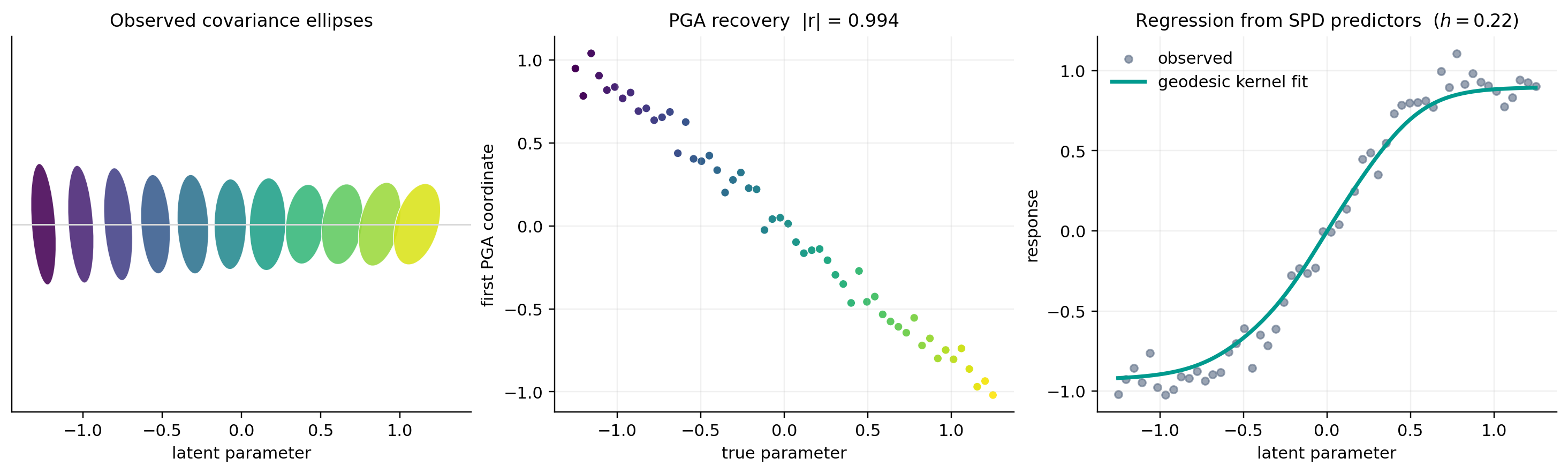
PGA explained variance: [0.9842 0.0093]
|correlation(parameter, PC1)|: 0.9935
selected bandwidth: 0.22
cross-validation MSE: [0.01802 0.02369 0.04745 0.11324 0.21139]
training RMSE: 0.1274

Visual report#

The left panel draws selected covariance ellipses along the generating path. The middle panel checks that PGA recovers the hidden progression, up to the arbitrary sign of an eigenvector. The right panel reports the fitted nonlinear response.

fig, axes = plt.subplots(1, 3, figsize=(13.2, 3.9), constrained_layout=True)
cmap = plt.get_cmap("viridis")
normalizer = plt.Normalize(float(t.min()), float(t.max()))

axes[0].axhline(0.0, color="0.85", linewidth=1)
for index in range(0, len(t), 5):
    matrix = np.asarray(covariances[index])
    values, vectors = np.linalg.eigh(matrix)
    order = np.argsort(values)[::-1]
    values, vectors = values[order], vectors[:, order]
    angle = np.degrees(np.arctan2(vectors[1, 0], vectors[0, 0]))
    ellipse = Ellipse(
        (float(t[index]), 0.0),
        width=0.18 * np.sqrt(values[0]),
        height=0.18 * np.sqrt(values[1]),
        angle=angle,
        facecolor=cmap(normalizer(float(t[index]))),
        edgecolor="white",
        linewidth=0.5,
        alpha=0.88,
    )
    axes[0].add_patch(ellipse)
axes[0].set(xlim=(-1.45, 1.45), ylim=(-0.34, 0.34), xlabel="latent parameter")
axes[0].set_title("Observed covariance ellipses")
axes[0].set_yticks([])

scatter = axes[1].scatter(
    np.asarray(t), np.asarray(pga.coordinates[:, 0]), c=np.asarray(t),
    cmap=cmap, s=25, edgecolor="white", linewidth=0.3,
)
axes[1].set(xlabel="true parameter", ylabel="first PGA coordinate")
axes[1].set_title(f"PGA recovery  |r| = {abs(correlation):.3f}")
axes[1].grid(alpha=0.18)

axes[2].scatter(np.asarray(t), np.asarray(response), s=20, color="#64748B", alpha=0.65, label="observed")
axes[2].plot(np.asarray(t_grid), np.asarray(prediction), color="#009A8E", linewidth=2.4, label="geodesic kernel fit")
axes[2].set(xlabel="latent parameter", ylabel="response")
axes[2].set_title(f"Regression from SPD predictors  ($h={bandwidth_selection.bandwidth:g}$)")
axes[2].legend(frameon=False, loc="upper left")
axes[2].grid(alpha=0.18)

output = next(
    path for path in (
        Path("../_static/tutorials/spd-pga-regression.png"),
        Path("docs/_static/tutorials/spd-pga-regression.png"),
        Path("_static/tutorials/spd-pga-regression.png"),
    )
    if path.parent.exists()
)
output.parent.mkdir(parents=True, exist_ok=True)
fig.savefig(output, bbox_inches="tight")
plt.show()

../_images/b5bbb4dee350a745fe0e001adbf6a9419d9e80a328a251f3f154b2485e50aa17.png

The analysis never vectorizes the covariance matrices by hand. Changing M changes the distance, mean, tangent metric, and therefore both fitted methods.

References#

[AFPA07]

Vincent Arsigny, Pierre Fillard, Xavier Pennec, and Nicholas Ayache. Geometric means in a novel vector space structure on symmetric positive-definite matrices. SIAM Journal on Matrix Analysis and Applications, 29(1):328–347, 2007. doi:10.1137/050637996.

[FLPJ04]

P. Thomas Fletcher, Conglin Lu, Stephen M. Pizer, and Sarang Joshi. Principal geodesic analysis for the study of nonlinear statistics of shape. IEEE Transactions on Medical Imaging, 23(8):995–1005, 2004. doi:10.1109/TMI.2004.831793.