Robust Location Summaries on the Circle

An average is not the only useful summary of manifold-valued observations. For points \(x_1,\ldots,x_n\) on a manifold, the Fréchet mean, geometric median, and minimum enclosing ball solve different problems:

\[ \widehat\mu=\arg\min_p\sum_i d(p,x_i)^2, \qquad \widehat m=\arg\min_p\sum_i d(p,x_i), \qquad (\widehat c,\widehat r)=\arg\min_{c,r}\{r:d(c,x_i)\leq r\}. \]

The mean emphasizes large residuals, the median is more resistant to isolated observations, and the enclosing ball controls the worst residual. GeoJAX computes all three from the same validated circular data [Fréchet, 1948, Karcher, 1977, Weiszfeld, 1937].

from pathlib import Path

import jax
jax.config.update("jax_enable_x64", True)
import jax.numpy as jnp
import matplotlib.pyplot as plt
import numpy as np

from geojax.geometry import Sphere
from geojax.learning import (
    frechet_mean,
    frechet_median,
    geodesic_interpolation,
    minimum_enclosing_ball,
    nearest_neighbors,
    pairwise_distances,
)

plt.rcParams.update({
    "figure.dpi": 220,
    "savefig.dpi": 320,
    "font.size": 10,
    "axes.titlesize": 11,
    "axes.spines.top": False,
    "axes.spines.right": False,
})

M = Sphere(size=2)
key = jax.random.key(401)
core_angles = 0.32 + 0.17 * jax.random.normal(key, (28,))
outlier_angles = jnp.array([-1.42, 1.82, 2.12])
angles = jnp.concatenate([core_angles, outlier_angles])
points = jnp.stack([jnp.cos(angles), jnp.sin(angles)], axis=-1)

mean = frechet_mean(M, points, maxiter=100, tol=1e-9)
median = frechet_median(M, points, maxiter=200, tol=1e-8)
ball = minimum_enclosing_ball(M, points, maxiter=500, tol=1e-8)

query_angle = -0.04
query = jnp.array([[jnp.cos(query_angle), jnp.sin(query_angle)]])
neighbors = nearest_neighbors(
    M, points, queries=query, n_neighbors=5, exclude_self=False
)

def point_angle(point):
    return float(jnp.arctan2(point[1], point[0]))

print(f"Fréchet mean angle:   {point_angle(mean.point): .4f}")
print(f"Fréchet median angle: {point_angle(median.point): .4f}")
print(f"enclosing center:     {point_angle(ball.center): .4f}")
print(f"enclosing radius:     {float(ball.radius): .4f}")
print("nearest sample indices:", np.asarray(neighbors.indices[0]))

Fréchet mean angle:    0.4068
Fréchet median angle:  0.3861
enclosing center:      0.3500
enclosing radius:      1.7700
nearest sample indices: [ 5 18  3  1 21]

Inspect the three objectives

The public result objects preserve both estimates and diagnostics. We evaluate the two location losses over the full angular chart and separately compare the ordered residuals of all three centers. The geodesic drawn from the enclosing center reaches its farthest observation through the public interpolation primitive.

angle_grid = jnp.linspace(-jnp.pi, jnp.pi, 500, endpoint=False)
grid_points = jnp.stack([jnp.cos(angle_grid), jnp.sin(angle_grid)], axis=-1)
grid_distances = pairwise_distances(M, grid_points, points)
mean_loss = jnp.mean(grid_distances**2, axis=1)
median_loss = jnp.mean(grid_distances, axis=1)

ball_distances = M.dist(ball.center, points)
farthest = points[int(jnp.argmax(ball_distances))]
ball_path = geodesic_interpolation(
    M, ball.center, farthest, jnp.linspace(0.0, 1.0, 90)
)

centers = {
    "mean": mean.point,
    "median": median.point,
    "enclosing": ball.center,
}
colors = {
    "mean": "#E45756",
    "median": "#009E8E",
    "enclosing": "#7C3AED",
}

Visual report

Open circles mark the five nearest neighbors of the query diamond. The loss panel shows why the median remains near the dense mode, while the sorted residual panel shows the enclosing center trading average fit for a smaller maximum distance.

fig, axes = plt.subplots(1, 3, figsize=(13.4, 4.0), constrained_layout=True)

circle = np.linspace(-np.pi, np.pi, 500)
axes[0].plot(np.cos(circle), np.sin(circle), color="0.80", linewidth=1.2)
axes[0].scatter(
    np.asarray(points[:-3, 0]), np.asarray(points[:-3, 1]),
    color="#64748B", s=28, alpha=0.72, label="main sample",
)
axes[0].scatter(
    np.asarray(points[-3:, 0]), np.asarray(points[-3:, 1]),
    color="#F59E0B", marker="x", s=55, linewidth=1.5, label="isolated points",
)
neighbor_indices = np.asarray(neighbors.indices[0])
axes[0].scatter(
    np.asarray(points[neighbor_indices, 0]), np.asarray(points[neighbor_indices, 1]),
    facecolors="none", edgecolors="#111827", s=82, linewidth=1.0,
    label="query neighbors",
)
axes[0].scatter(*np.asarray(query[0]), marker="D", color="#111827", s=55, label="query")
for name, center in centers.items():
    axes[0].scatter(
        *np.asarray(center), marker="*", color=colors[name], edgecolor="white",
        linewidth=0.6, s=180, label=name,
    )
axes[0].plot(
    np.asarray(ball_path[:, 0]), np.asarray(ball_path[:, 1]),
    color=colors["enclosing"], linestyle="--", linewidth=2.0,
)
axes[0].set(aspect="equal", xlim=(-1.12, 1.12), ylim=(-1.12, 1.12))
axes[0].set_title("Data and intrinsic summaries")
axes[0].legend(frameon=False, fontsize=8, loc="center")

axes[1].plot(
    np.asarray(angle_grid), np.asarray(mean_loss - jnp.min(mean_loss)),
    color=colors["mean"], linewidth=2.1, label="squared-distance loss",
)
axes[1].plot(
    np.asarray(angle_grid), np.asarray(median_loss - jnp.min(median_loss)),
    color=colors["median"], linewidth=2.1, label="distance loss",
)
for name in ("mean", "median"):
    axes[1].axvline(point_angle(centers[name]), color=colors[name], linestyle=":")
axes[1].set(
    title="Location objectives",
    xlabel="candidate angle",
    ylabel="loss above its minimum",
    xlim=(-np.pi, np.pi),
)
axes[1].grid(alpha=0.18)
axes[1].legend(frameon=False)

rank = np.arange(1, len(points) + 1)
for name, center in centers.items():
    residuals = np.sort(np.asarray(M.dist(center, points)))
    axes[2].plot(rank, residuals, color=colors[name], linewidth=2.0, label=name)
axes[2].axhline(float(ball.radius), color=colors["enclosing"], linestyle="--", alpha=0.7)
axes[2].set(
    title="Ordered geodesic residuals",
    xlabel="ordered observation",
    ylabel="distance from center",
)
axes[2].grid(alpha=0.18)
axes[2].legend(frameon=False)

output = next(
    path for path in (
        Path("../_static/tutorials/robust-spherical-summaries.png"),
        Path("docs/_static/tutorials/robust-spherical-summaries.png"),
        Path("_static/tutorials/robust-spherical-summaries.png"),
    )
    if path.parent.exists()
)
output.parent.mkdir(parents=True, exist_ok=True)
fig.savefig(output, bbox_inches="tight")
plt.show()

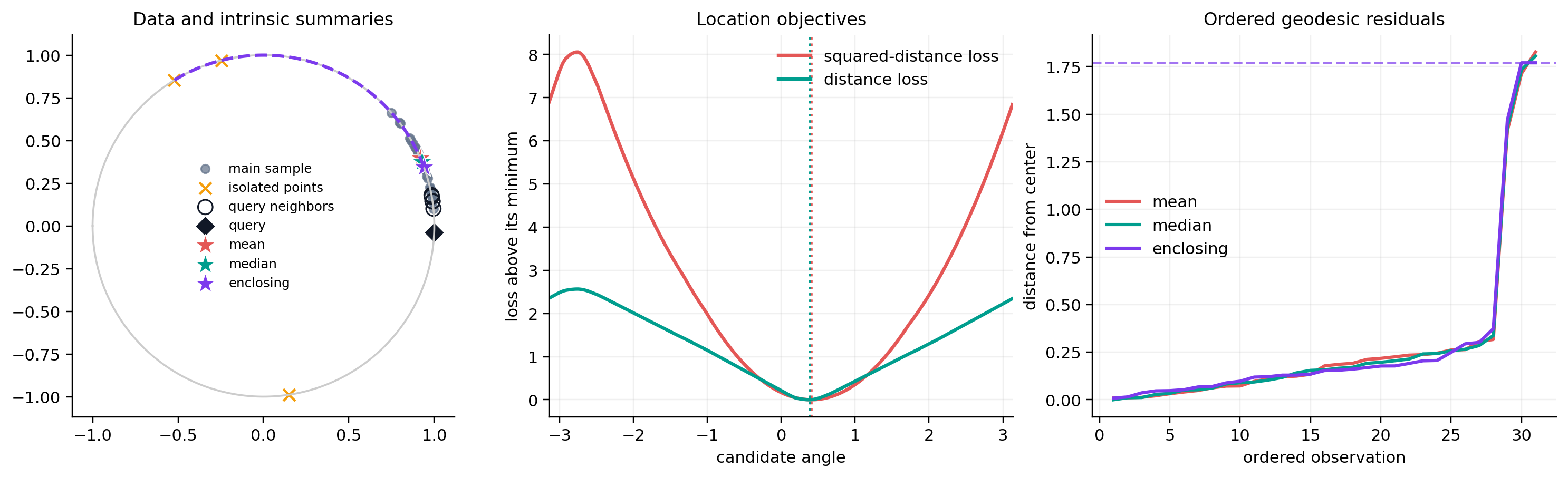
None of these summaries is universally preferable. The objective should match the scientific question: central squared error, robust central location, or a worst-case coverage radius. Near a cut locus, any intrinsic location routine also inherits the branch convention of the selected geometry.

References

[Frechet48]

Maurice Fréchet. Les éléments aléatoires de nature quelconque dans un espace distancié. Annales de l'Institut Henri Poincaré, 10(4):215–310, 1948. URL: https://www.numdam.org/item/AIHP_1948__10_4_215_0/.

[Kar77]

Hermann Karcher. Riemannian center of mass and mollifier smoothing. Communications on Pure and Applied Mathematics, 30(5):509–541, 1977. doi:10.1002/cpa.3160300502.

[Wei37]

Endre Weiszfeld. Sur le point pour lequel la somme des distances de n points donnés est minimum. Tohoku Mathematical Journal, 43:355–386, 1937.