Regression with Circular Responses

When a response lies on a manifold, an ordinary componentwise fit can leave the sample space. A geodesic regression instead uses

\[ \widehat Y(t)=\operatorname{Exp}_{p}\!\left((t-\overline t)v\right), \]

with \(p\in\mathcal M\) and \(v\in T_p\mathcal M\). This is the intrinsic analogue of a straight line [Fletcher, 2013]. Local Fréchet regression is more flexible: at each query it minimizes a locally weighted squared- distance objective [Petersen and Müller, 2019].

We generate circular responses along a mildly nonlinear trajectory, then compare the parametric geodesic and local-linear fits.

from pathlib import Path

import jax
jax.config.update("jax_enable_x64", True)
import jax.numpy as jnp
import matplotlib.pyplot as plt
import numpy as np

from geojax.geometry import Sphere
from geojax.learning import (
    bootstrap_frechet_mean,
    geodesic_regression,
    local_polynomial_regression,
)

plt.rcParams.update({
    "figure.dpi": 220,
    "savefig.dpi": 320,
    "font.size": 10,
    "axes.titlesize": 11,
    "axes.spines.top": False,
    "axes.spines.right": False,
})

M = Sphere(size=2)
predictors = jnp.linspace(-1.0, 1.0, 19)
true_angles = 0.25 + 0.92 * predictors + 0.18 * jnp.sin(jnp.pi * predictors)
noise = 0.07 * jax.random.normal(jax.random.key(520), predictors.shape)
observed_angles = true_angles + noise

def on_circle(angles):
    return jnp.stack([jnp.cos(angles), jnp.sin(angles)], axis=-1)

responses = on_circle(observed_angles)
geodesic = geodesic_regression(M, predictors, responses, maxiter=100, tol=1e-8)
local = local_polynomial_regression(
    M,
    predictors,
    responses,
    bandwidth=0.38,
    degree=1,
    maxiter=50,
    tol=1e-7,
)

grid = jnp.linspace(-1.0, 1.0, 41)
geodesic_predictions = geodesic.predict(grid)
local_predictions = local.predict(grid)
truth = on_circle(0.25 + 0.92 * grid + 0.18 * jnp.sin(jnp.pi * grid))

geodesic_error = jnp.mean(M.dist(geodesic_predictions, truth) ** 2)
local_error = jnp.mean(M.dist(local_predictions, truth) ** 2)
print(f"geodesic fit MSE:    {float(geodesic_error):.6f}")
print(f"local-linear MSE:    {float(local_error):.6f}")

geodesic fit MSE:    0.008941
local-linear MSE:    0.005898

Bootstrap a central circular response

The bootstrap result below is a percentile ball formed from replicate Fréchet means. It describes empirical estimator dispersion; it is not a curvature-corrected confidence region.

bootstrap = bootstrap_frechet_mean(
    M,
    responses,
    n_bootstrap=30,
    confidence_level=0.9,
    key=jax.random.key(521),
    maxiter=60,
    tol=1e-7,
)

def angles_of(points):
    return np.unwrap(np.arctan2(np.asarray(points[..., 1]), np.asarray(points[..., 0])))

print(f"90% bootstrap radius: {float(bootstrap.confidence_radius):.4f} radians")

90% bootstrap radius: 0.2154 radians

Visual report

The left panel keeps every estimate on the circle. The middle panel unwraps the same points only for plotting against the scalar predictor. The last panel shows bootstrap mean angles relative to the original estimate.

fig, axes = plt.subplots(1, 3, figsize=(13.4, 4.0), constrained_layout=True)
circle = np.linspace(-np.pi, np.pi, 600)
axes[0].plot(np.cos(circle), np.sin(circle), color="0.82", linewidth=1.1)
axes[0].scatter(
    np.asarray(responses[:, 0]), np.asarray(responses[:, 1]),
    c=np.asarray(predictors), cmap="viridis", s=36, edgecolor="white", linewidth=0.4,
    label="observations",
)
axes[0].plot(
    np.asarray(geodesic_predictions[:, 0]), np.asarray(geodesic_predictions[:, 1]),
    color="#E45756", linewidth=2.2, linestyle="--", label="geodesic fit",
)
axes[0].plot(
    np.asarray(local_predictions[:, 0]), np.asarray(local_predictions[:, 1]),
    color="#009E8E", linewidth=2.2, label="local-linear fit",
)
axes[0].scatter(
    *np.asarray(bootstrap.estimate), marker="*", s=190, color="#7C3AED",
    edgecolor="white", linewidth=0.6, label="Fréchet mean",
)
axes[0].set(aspect="equal", xlim=(-1.1, 1.1), ylim=(-1.1, 1.1), title="Fits remain on the circle")
axes[0].set_xticks([])
axes[0].set_yticks([])
axes[0].legend(frameon=False, fontsize=8, loc="center")

axes[1].scatter(
    np.asarray(predictors), np.asarray(observed_angles),
    color="#64748B", s=30, alpha=0.78, label="observed",
)
axes[1].plot(np.asarray(grid), angles_of(truth), color="#111827", linewidth=1.8, label="truth")
axes[1].plot(
    np.asarray(grid), angles_of(geodesic_predictions),
    color="#E45756", linestyle="--", linewidth=2.0, label="geodesic",
)
axes[1].plot(
    np.asarray(grid), angles_of(local_predictions),
    color="#009E8E", linewidth=2.0, label="local linear",
)
axes[1].set(title="Angular chart for comparison", xlabel="predictor", ylabel="unwrapped angle")
axes[1].grid(alpha=0.18)
axes[1].legend(frameon=False, fontsize=8)

replicate_angles = np.arctan2(
    np.asarray(bootstrap.replicates[:, 1]), np.asarray(bootstrap.replicates[:, 0])
)
estimate_angle = float(jnp.arctan2(bootstrap.estimate[1], bootstrap.estimate[0]))
centered_replicates = np.angle(np.exp(1j * (replicate_angles - estimate_angle)))
axes[2].hist(centered_replicates, bins=12, color="#7C3AED", alpha=0.72, edgecolor="white")
axes[2].axvline(-float(bootstrap.confidence_radius), color="#111827", linestyle="--")
axes[2].axvline(float(bootstrap.confidence_radius), color="#111827", linestyle="--")
axes[2].set(
    title="Bootstrap Fréchet-mean displacement",
    xlabel="signed angular displacement",
    ylabel="replicates",
)
axes[2].grid(axis="y", alpha=0.18)

output = next(
    path for path in (
        Path("../_static/tutorials/manifold-response-regression.png"),
        Path("docs/_static/tutorials/manifold-response-regression.png"),
        Path("_static/tutorials/manifold-response-regression.png"),
    )
    if path.parent.exists()
)
output.parent.mkdir(parents=True, exist_ok=True)
fig.savefig(output, bbox_inches="tight")
plt.show()

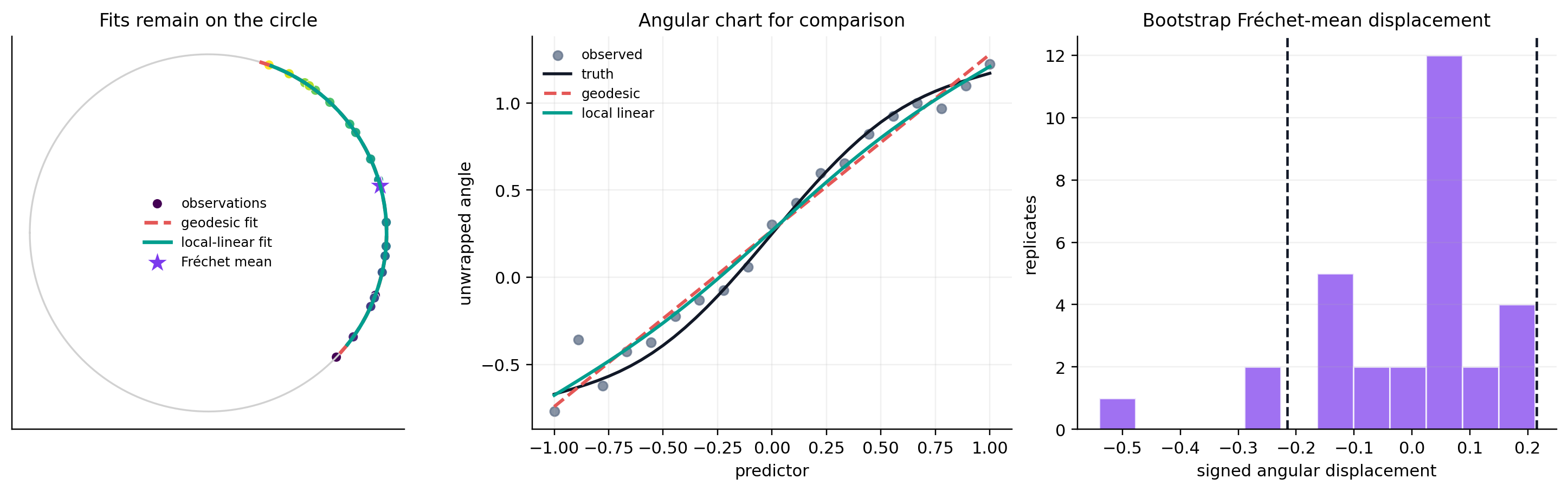
The geodesic model is concise and interpretable, while the local fit tracks the non-geodesic bend. Near a cut locus, both inherit the selected logarithm branch; bandwidth and chart coverage are therefore geometric modeling choices.

References

[Fle13]

P. Thomas Fletcher. Geodesic regression and the theory of least squares on Riemannian manifolds. International Journal of Computer Vision, 105(2):171–185, 2013. doi:10.1007/s11263-012-0591-y.

[PMuller19]

Alexander Petersen and Hans-Georg Müller. Fréchet regression for random objects with Euclidean predictors. The Annals of Statistics, 47(2):691–719, 2019. doi:10.1214/17-AOS1624.