Wrapped geodesics on the flat torus

The flat torus \(\mathbb T^2=S^1\times S^1\) can be represented by two angles in \([-\pi,\pi)\). Its logarithm chooses the shortest wrapped angular difference,

\[ \operatorname{Log}_x(y)=\operatorname{wrap}(y-x), \]

and the exponential map adds that tangent vector modulo \(2\pi\). A shortest path can therefore cross the edge of the angular coordinate square while remaining smooth on the torus itself. The construction is the product metric and quotient representation of a flat Riemannian manifold [do Carmo, 1992].

import jax
jax.config.update("jax_enable_x64", True)
import jax.numpy as jnp
import matplotlib.pyplot as plt
import numpy as np

from geojax.geometry import Torus

plt.rcParams.update({
    "figure.dpi": 200,
    "savefig.dpi": 240,
    "font.size": 11,
    "axes.titlesize": 12,
    "axes.labelsize": 11,
    "xtick.labelsize": 10,
    "ytick.labelsize": 10,
    "legend.fontsize": 9,
    "axes.spines.top": False,
    "axes.spines.right": False,
})

M = Torus(size=2)
x = jnp.array([2.75, 2.45])
y = jnp.array([-2.60, -2.20])
velocity = M.log(x, y)
times = jnp.linspace(0.0, 1.0, 180)
path = jax.vmap(lambda time: M.exp(x, time * velocity))(times)

print("shortest wrapped displacement:", velocity)
print("intrinsic distance:", float(M.dist(x, y)))
print("unwrapped Euclidean difference:", float(jnp.linalg.norm(y - x)))
print("endpoint error:", float(M.dist(path[-1], y)))

shortest wrapped displacement: [0.93318531 1.63318531]
intrinsic distance: 1.8809915111778515
unwrapped Euclidean difference: 7.088370757797591
endpoint error: 4.440892098500626e-16

Compare intrinsic and coordinate views

The familiar embedded torus is only a visualization of this flat product geometry; its induced surface metric is different. It is nevertheless useful for seeing that the apparent jumps in angular coordinates are not breaks in the path.

def embed_torus(angles, major_radius=2.0, minor_radius=0.72):
    theta = angles[..., 0]
    phi = angles[..., 1]
    radius = major_radius + minor_radius * np.cos(phi)
    return np.stack([
        radius * np.cos(theta),
        radius * np.sin(theta),
        minor_radius * np.sin(phi),
    ], axis=-1)


theta_grid = np.linspace(-np.pi, np.pi, 90)
phi_grid = np.linspace(-np.pi, np.pi, 55)
Theta, Phi = np.meshgrid(theta_grid, phi_grid)
surface = embed_torus(np.stack([Theta, Phi], axis=-1))
embedded_path = embed_torus(np.asarray(path))
embedded_endpoints = embed_torus(np.asarray(jnp.stack([x, y])))

fig = plt.figure(figsize=(11.5, 4.8), constrained_layout=True)
ax_torus = fig.add_subplot(1, 2, 1, projection="3d")
ax_angles = fig.add_subplot(1, 2, 2)

ax_torus.plot_surface(
    surface[..., 0], surface[..., 1], surface[..., 2],
    color="#D9ECEB", alpha=0.55, linewidth=0, antialiased=True,
)
ax_torus.plot(*embedded_path.T, color="#D97706", linewidth=3.0)
ax_torus.scatter(*embedded_endpoints.T, color=["#007C83", "#7C3AED"], s=58)
ax_torus.set(title="Continuous path on the torus", xlabel="$X$", ylabel="$Y$", zlabel="$Z$")
ax_torus.set_box_aspect((1, 1, 0.5))
ax_torus.view_init(elev=27, azim=-46)

ax_angles.plot(path[:, 0], path[:, 1], color="#D97706", linewidth=2.2)
ax_angles.scatter([x[0], y[0]], [x[1], y[1]], color=["#007C83", "#7C3AED"], s=55)
ax_angles.set(
    title="The same path in wrapped coordinates",
    xlabel=r"$\theta_1$",
    ylabel=r"$\theta_2$",
    xlim=(-np.pi, np.pi),
    ylim=(-np.pi, np.pi),
    xticks=[-np.pi, 0.0, np.pi],
    yticks=[-np.pi, 0.0, np.pi],
    xticklabels=[r"$-\pi$", "$0$", r"$\pi$"],
    yticklabels=[r"$-\pi$", "$0$", r"$\pi$"],
)
ax_angles.grid(alpha=0.22)

plt.show()

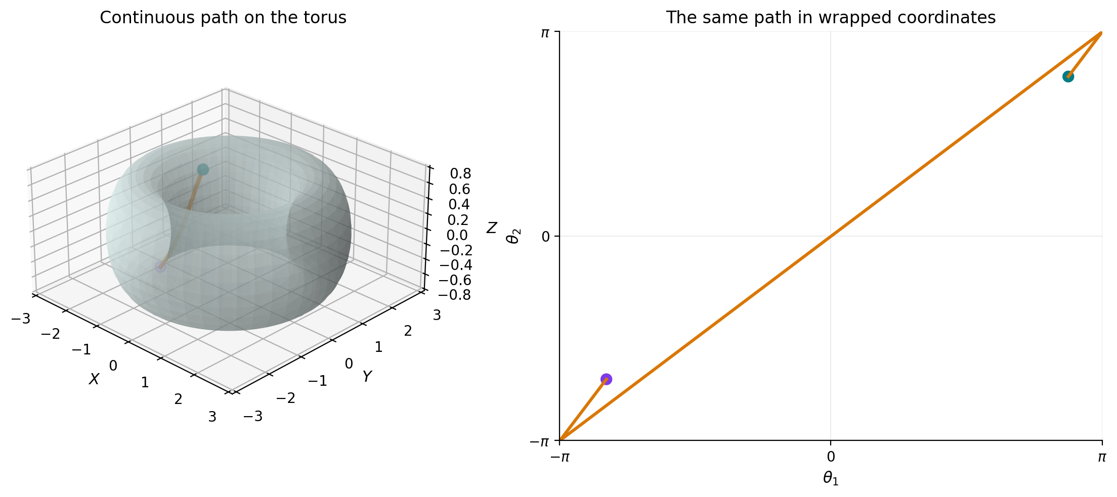
The broken appearance in the coordinate square is the expected effect of choosing one representative for each periodic angle. Torus.log selects the short branch automatically, and Torus.exp wraps every intermediate point.

What to try next

• Move one endpoint until a coordinate difference is exactly \(\pi\).

• Plot several tangent directions from the same point.

• Use Product to combine a torus state with a sphere or matrix geometry.

References

[dC92]

Manfredo P. do Carmo. Riemannian Geometry. Birkhäuser, 1992. doi:10.1007/978-1-4757-2201-7.