Robust and Scalable Circular Summaries

Full-batch Fréchet means optimize a global sample objective. Streaming and mini-batch summaries replace that optimization with log-map updates, which is useful for larger samples but introduces order and step-size effects. Robust estimators change the objective itself by trimming or downweighting large geodesic residuals [Bonnabel, 2013, Fletcher et al., 2009].

This tutorial places those two questions in one contaminated circular sample: how much computation is used, and how much influence is assigned to isolated observations?

from pathlib import Path

import jax
jax.config.update("jax_enable_x64", True)
import jax.numpy as jnp
import matplotlib.pyplot as plt
import numpy as np

from geojax.geometry import Sphere
from geojax.learning import (
    frechet_mean,
    geodesic_m_estimator,
    geodesic_spatial_depth,
    minibatch_frechet_mean,
    minibatch_kmeans,
    streaming_frechet_mean,
    trimmed_frechet_mean,
)

plt.rcParams.update({
    "figure.dpi": 220,
    "savefig.dpi": 320,
    "font.size": 10,
    "axes.titlesize": 11,
    "axes.spines.top": False,
    "axes.spines.right": False,
})

M = Sphere(size=2)
key_a, key_b = jax.random.split(jax.random.key(540))
angles = jnp.concatenate([
    -0.35 + 0.13 * jax.random.normal(key_a, (26,)),
    0.62 + 0.14 * jax.random.normal(key_b, (20,)),
    jnp.array([2.35, 2.65, -2.55]),
])

def on_circle(theta):
    return jnp.stack([jnp.cos(theta), jnp.sin(theta)], axis=-1)

data = on_circle(angles)
full = frechet_mean(M, data, maxiter=100, tol=1e-8)
forward = streaming_frechet_mean(M, data)
reverse = streaming_frechet_mean(M, data[::-1])
mini = minibatch_frechet_mean(
    M, data, batch_size=8, epochs=10, key=jax.random.key(541),
    learning_rate=0.7, decay=0.15,
)
trimmed = trimmed_frechet_mean(M, data, trim_fraction=0.16, maxiter=30)
huber = geodesic_m_estimator(M, data, loss="huber", maxiter=30)
cauchy = geodesic_m_estimator(M, data, loss="cauchy", maxiter=30)

clusters = minibatch_kmeans(
    M, data, n_clusters=2, batch_size=8, epochs=12,
    key=jax.random.key(542), learning_rate=0.6, decay=0.08,
)

def point_angle(point):
    return float(jnp.arctan2(point[1], point[0]))

for name, point in (
    ("full mean", full.point),
    ("stream forward", forward.point),
    ("stream reverse", reverse.point),
    ("mini-batch", mini.point),
    ("trimmed", trimmed.point),
    ("Huber", huber.point),
    ("Cauchy", cauchy.point),
):
    print(f"{name:15s}: angle = {point_angle(point): .4f}")

full mean      : angle =  0.1184
stream forward : angle =  0.1184
stream reverse : angle =  0.2466
mini-batch     : angle =  0.1506
trimmed        : angle = -0.0117
Huber          : angle =  0.0919
Cauchy         : angle =  0.0821

Depth and residual influence

Intrinsic spatial depth averages unit log directions. It is high where those directions balance and decreases toward peripheral locations:

\[ D(x)=1-\left\|\frac1n\sum_i \frac{\operatorname{Log}_x(x_i)}{d(x,x_i)}\right\|_x. \]

grid_angles = jnp.linspace(-jnp.pi, jnp.pi, 181, endpoint=False)
grid_points = on_circle(grid_angles)
depths = geodesic_spatial_depth(M, grid_points, data)

summaries = {
    "full": full.point,
    "forward": forward.point,
    "reverse": reverse.point,
    "mini-batch": mini.point,
    "trimmed": trimmed.point,
    "Huber": huber.point,
    "Cauchy": cauchy.point,
}
colors = {
    "full": "#111827",
    "forward": "#2563EB",
    "reverse": "#7C3AED",
    "mini-batch": "#F59E0B",
    "trimmed": "#009E8E",
    "Huber": "#E45756",
    "Cauchy": "#8B5CF6",
}

fig, axes = plt.subplots(1, 3, figsize=(13.3, 4.0), constrained_layout=True)
circle = np.linspace(-np.pi, np.pi, 600)
axes[0].plot(np.cos(circle), np.sin(circle), color="0.82", linewidth=1.1)
axes[0].scatter(
    np.asarray(data[:-3, 0]), np.asarray(data[:-3, 1]),
    color="#64748B", s=27, alpha=0.72, label="main sample",
)
axes[0].scatter(
    np.asarray(data[-3:, 0]), np.asarray(data[-3:, 1]),
    color="#F59E0B", marker="x", s=58, linewidth=1.6, label="contamination",
)
for name, point in summaries.items():
    axes[0].scatter(
        *np.asarray(point), marker="*", s=145, color=colors[name],
        edgecolor="white", linewidth=0.5, label=name,
    )
axes[0].set(aspect="equal", xlim=(-1.12, 1.12), ylim=(-1.12, 1.12), title="Location estimates")
axes[0].set_xticks([])
axes[0].set_yticks([])
axes[0].legend(frameon=False, fontsize=7, loc="center")

axes[1].plot(np.asarray(grid_angles), np.asarray(depths), color="#009E8E", linewidth=2.1)
for name in ("full", "trimmed", "Huber", "Cauchy"):
    axes[1].axvline(point_angle(summaries[name]), color=colors[name], linestyle=":", label=name)
axes[1].set(
    title="Intrinsic spatial depth",
    xlabel="candidate angle",
    ylabel="depth",
    xlim=(-np.pi, np.pi),
    ylim=(-0.02, 1.02),
)
axes[1].grid(alpha=0.18)
axes[1].legend(frameon=False, fontsize=8)

labels = np.asarray(clusters.labels)
axes[2].scatter(
    np.arange(len(data)), np.asarray(angles),
    c=labels, cmap="coolwarm", s=35, edgecolor="white", linewidth=0.35,
)
history = np.asarray(clusters.diagnostics["objective_history"])
inset = axes[2].inset_axes([0.55, 0.55, 0.4, 0.36])
inset.plot(np.arange(1, len(history) + 1), history, marker="o", color="#7C3AED")
inset.set_title("mini-batch objective", fontsize=8)
inset.tick_params(labelsize=7)
axes[2].set(
    title="Mini-batch intrinsic k-means",
    xlabel="observation order",
    ylabel="angle",
)
axes[2].grid(alpha=0.18)

output = next(
    path for path in (
        Path("../_static/tutorials/robust-scalable-learning.png"),
        Path("docs/_static/tutorials/robust-scalable-learning.png"),
        Path("_static/tutorials/robust-scalable-learning.png"),
    )
    if path.parent.exists()
)
output.parent.mkdir(parents=True, exist_ok=True)
fig.savefig(output, bbox_inches="tight")
plt.show()

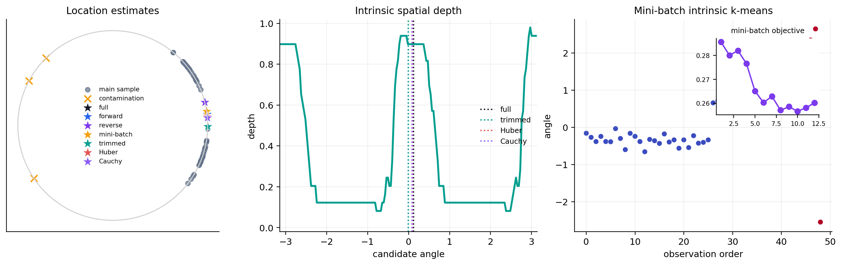
The forward and reversed streaming estimates need not coincide on a curved space. Robust estimates answer a different question: they deliberately reduce the influence of large residuals. Neither approximation error nor robustness should be inferred from the method name alone; inspect the returned objective, weights, retained set, and update history.

References

[Bon13]

Silvère Bonnabel. Stochastic gradient descent on Riemannian manifolds. IEEE Transactions on Automatic Control, 58(9):2217–2229, 2013. doi:10.1109/TAC.2013.2254619.

[FVJ09]

P. Thomas Fletcher, Suresh Venkatasubramanian, and Sarang Joshi. The geometric median on Riemannian manifolds with application to robust atlas estimation. NeuroImage, 45(1, Supplement 1):S143–S152, 2009. doi:10.1016/j.neuroimage.2008.10.052.