

Comparing clustering methods on a flat torus#
Clustering manifold-valued data is not one algorithm with interchangeable names. Intrinsic k-means minimizes squared distances to Frechet centers; k-medoids restricts representatives to observed points; hierarchical and spectral methods use only the distance matrix; mean shift searches for density modes; and competitive quantization updates prototypes online. Their outputs can differ even when every method uses the same geodesic distance.
We compare these objectives on the flat two-torus \(T^2=(\mathbb R/2\pi\mathbb Z)^2\). GeoJAX represents a point by wrapped angles \(\theta=(\theta_1,\theta_2)\in[-\pi,\pi)^2\), with
Thus opposite edges of the displayed square are identified. Several groups below cross those edges, making ordinary Euclidean clustering of the angle table inappropriate. The methods follow Lloyd [1982], Kaufman and Rousseeuw [1990], Zelnik-Manor and Perona [2005], Comaniciu and Meer [2002], and the Riemannian quantization method of Le Brigant and Puechmorel [2019]. The coreset heuristic is adapted from Bachem et al. [2018].
from dataclasses import replace
from pathlib import Path

import jax
jax.config.update("jax_enable_x64", True)
import jax.numpy as jnp
import matplotlib.pyplot as plt
import numpy as np

from geojax.geometry import Torus
from geojax.learning import (
    agglomerative_clustering,
    competitive_quantization,
    kmeans,
    kmedoids,
    lightweight_coreset,
    mean_shift,
    pairwise_distances,
    spectral_clustering,
)

plt.rcParams.update({
    "figure.dpi": 220,
    "savefig.dpi": 320,
    "font.size": 9.5,
    "axes.titlesize": 10.5,
    "axes.spines.top": False,
    "axes.spines.right": False,
})

M = Torus(size=2)
cluster_centers = jnp.array([
    [-3.05, 1.80],
    [0.05, -0.18],
    [1.80, 3.02],
])
cluster_scales = jnp.array([
    [0.18, 0.16],
    [0.23, 0.18],
    [0.16, 0.19],
])
keys = jax.random.split(jax.random.key(831), 3)
points = M.project(jnp.concatenate([
    center + scale * jax.random.normal(key, shape=(14, 2))
    for center, scale, key in zip(cluster_centers, cluster_scales, keys)
]))

full_kmeans = kmeans(
    M, points, n_clusters=3, key=jax.random.key(1), n_init=3,
    maxiter=35, center_maxiter=25,
)
medoids = kmedoids(
    M, points, n_clusters=3, key=jax.random.key(2), maxiter=35,
)
hierarchy = agglomerative_clustering(
    M, points, n_clusters=3, linkage="average",
)
spectral = spectral_clustering(
    M,
    points,
    n_clusters=3,
    key=jax.random.key(3),
    affinity="self_tuning",
    n_neighbors=6,
    maxiter=40,
)
modes = mean_shift(
    M, points, bandwidth=0.42, merge_tol=0.50, maxiter=40,
)
quantized = competitive_quantization(
    M,
    points,
    n_clusters=3,
    key=jax.random.key(4),
    epochs=12,
    initial_gain=0.45,
)

coreset = lightweight_coreset(
    M, points, size=16, key=jax.random.key(5),
)
coreset_kmeans = kmeans(
    M,
    coreset.points,
    n_clusters=3,
    sample_weight=coreset.weights,
    key=jax.random.key(6),
    n_init=2,
    maxiter=35,
    center_maxiter=25,
)
coreset_labels = jnp.argmin(
    pairwise_distances(M, points, coreset_kmeans.centers), axis=1,
)
coreset_kmeans = replace(coreset_kmeans, labels=coreset_labels)

results = {
    "Intrinsic k-means": full_kmeans,
    "k-medoids": medoids,
    "Average linkage": hierarchy,
    "Spectral": spectral,
    "Mean shift": modes,
    "Competitive quantization": quantized,
    "Coreset k-means": coreset_kmeans,
}

for name, result in results.items():
    n_found = int(jnp.unique(result.labels).size)
    print(
        f"{name:25s} clusters={n_found:2d}  "
        f"iterations={result.iterations:3d}  objective={float(result.objective):.5f}"
    )
Intrinsic k-means         clusters= 3  iterations=  2  objective=0.05035
k-medoids                 clusters= 3  iterations=  2  objective=0.20311
Average linkage           clusters= 3  iterations= 41  objective=11.88972
Spectral                  clusters= 3  iterations= 40  objective=0.05035
Mean shift                clusters= 3  iterations= 11  objective=0.05044
Competitive quantization  clusters= 3  iterations= 12  objective=0.05405
Coreset k-means           clusters= 3  iterations=  2  objective=0.05490
The reported objectives are method-specific: a linkage sum is not directly comparable with squared quantization error or a medoid distance. The visual partitions and representative points are the meaningful comparison here.
Visual report#
The dashed boundary is a coordinate cut, not a geometric boundary. A cluster split between the top and bottom or left and right edges remains contiguous on \(T^2\). The first panel shows the coreset; larger rings indicate repeated selections. Stars mark representatives when a method returns centers or medoids.
palette = np.array(["#E45756", "#009E8E", "#7C3AED", "#F59E0B", "#2563EB"])


def setup_torus_chart(axis, title):
    axis.set(
        aspect="equal",
        xlim=(-np.pi - 0.18, np.pi + 0.18),
        ylim=(-np.pi - 0.18, np.pi + 0.18),
        title=title,
        xlabel=r"$\theta_1$",
        ylabel=r"$\theta_2$",
        xticks=[-np.pi, 0.0, np.pi],
        yticks=[-np.pi, 0.0, np.pi],
        xticklabels=[r"$-\pi$", "$0$", r"$\pi$"],
        yticklabels=[r"$-\pi$", "$0$", r"$\pi$"],
    )
    axis.plot(
        [-np.pi, np.pi, np.pi, -np.pi, -np.pi],
        [-np.pi, -np.pi, np.pi, np.pi, -np.pi],
        color="#475569", linestyle="--", linewidth=1.0,
    )
    axis.grid(alpha=0.14)


def draw_partition(axis, result, title):
    labels = np.asarray(result.labels)
    setup_torus_chart(
        axis, f"{title}\n$k={len(np.unique(labels))}$",
    )
    axis.scatter(
        np.asarray(points[:, 0]), np.asarray(points[:, 1]),
        c=palette[labels % len(palette)], s=31,
        edgecolor="white", linewidth=0.35,
    )
    centers = getattr(result, "centers", None)
    if centers is not None:
        centers = np.asarray(centers)
        axis.scatter(
            centers[:, 0], centers[:, 1], marker="*", s=165,
            color="#111827", edgecolor="white", linewidth=0.6, zorder=5,
        )


fig, axes = plt.subplots(2, 4, figsize=(13.0, 7.0), constrained_layout=True)
axes = axes.ravel()

setup_torus_chart(axes[0], "Lightweight coreset")
axes[0].scatter(
    np.asarray(points[:, 0]), np.asarray(points[:, 1]),
    color="#94A3B8", s=22, alpha=0.55,
)
unique_indices, selection_counts = np.unique(
    np.asarray(coreset.indices), return_counts=True,
)
axes[0].scatter(
    np.asarray(points[unique_indices, 0]),
    np.asarray(points[unique_indices, 1]),
    facecolors="none", edgecolors="#E45756",
    s=45 + 30 * selection_counts, linewidth=1.3,
)

for axis, (name, result) in zip(axes[1:], results.items()):
    draw_partition(axis, result, name)

output = next(
    path for path in (
        Path("../_static/tutorials/clustering-comparison.png"),
        Path("docs/_static/tutorials/clustering-comparison.png"),
        Path("_static/tutorials/clustering-comparison.png"),
    )
    if path.parent.exists()
)
output.parent.mkdir(parents=True, exist_ok=True)
fig.savefig(output, bbox_inches="tight")
plt.show()
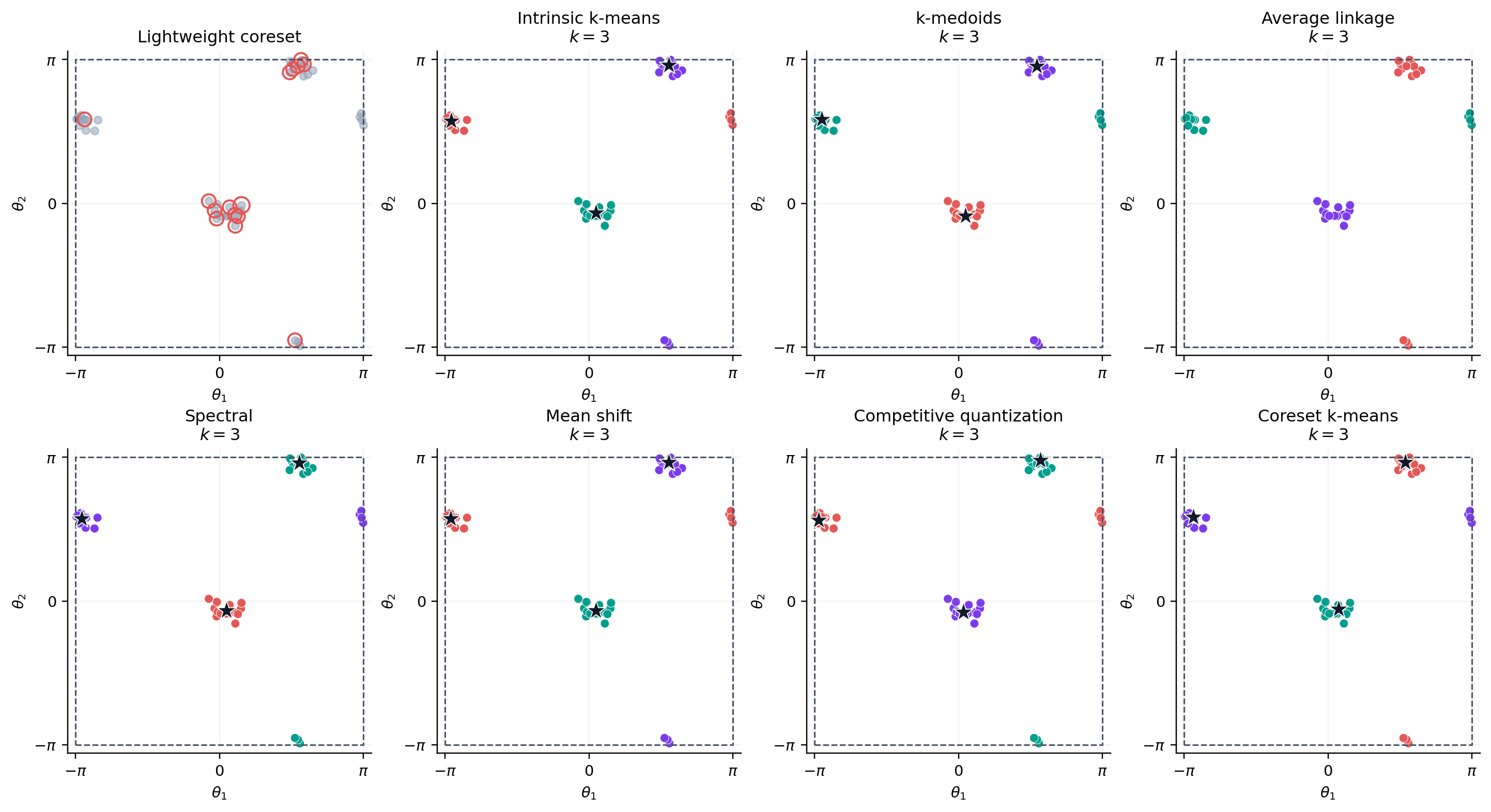
K-means, mean shift, and competitive quantization require logarithmic and exponential maps because they update manifold representatives. Medoids, hierarchy, and spectral clustering need only exact distances. The torus makes the distinction visible: methods must respect edge identification either through the intrinsic updates or through their distance matrix.
References#
Olivier Bachem, Mario Lucic, and Andreas Krause. Scalable k-Means clustering via lightweight coresets. In Proceedings of the 24th ACM SIGKDD International Conference on Knowledge Discovery and Data Mining, 1119–1127. 2018. doi:10.1145/3219819.3219973.
Dorin Comaniciu and Peter Meer. Mean shift: a robust approach toward feature space analysis. IEEE Transactions on Pattern Analysis and Machine Intelligence, 24(5):603–619, 2002. doi:10.1109/34.1000236.
Leonard Kaufman and Peter J. Rousseeuw. Finding Groups in Data: An Introduction to Cluster Analysis. John Wiley and Sons, New York, 1990. doi:10.1002/9780470316801.
Alice Le Brigant and Stéphane Puechmorel. Quantization and clustering on Riemannian manifolds with an application to air traffic analysis. Journal of Multivariate Analysis, 173:685–703, 2019. doi:10.1016/j.jmva.2019.05.008.
Stuart P. Lloyd. Least squares quantization in PCM. IEEE Transactions on Information Theory, 28(2):129–137, 1982. doi:10.1109/TIT.1982.1056489.
Lihi Zelnik-Manor and Pietro Perona. Self-tuning spectral clustering. In Advances in Neural Information Processing Systems, volume 17, 1601–1608. 2005.