Classification with Manifold-Valued Predictors

Suppose each predictor is a point \(x\in\mathcal M\), rather than a vector in a chosen coordinate chart. Two natural classifiers use only the intrinsic distance:

\[ \widehat c_{\mathrm{centroid}}(x) =\arg\min_c d(x,\widehat\mu_c), \qquad \widehat c_{\mathrm{kNN}}(x) =\operatorname{vote}\{y_i:i\in N_k(x)\}. \]

Tangent-space classifiers make a stronger local approximation. GeoJAX maps training logarithms at a Fréchet mean into a metric-orthonormal basis, then fits multinomial logistic regression or regularized discriminant analysis. The basis uses the Riemannian inner product and therefore also works for SPD and Product metrics that are not ambient Frobenius metrics. Distance-to-mean and tangent-coordinate classifiers are standard geometric learning patterns [Barachant et al., 2012, Fréchet, 1948].

We compare all four strategies on noisy circular observations.

from pathlib import Path

import jax
jax.config.update("jax_enable_x64", True)
import jax.numpy as jnp
import matplotlib.pyplot as plt
import numpy as np

from geojax.geometry import Sphere
from geojax.learning import (
    knn_classifier,
    nearest_centroid_classifier,
    tangent_space_discriminant_analysis,
    tangent_space_logistic_regression,
)

plt.rcParams.update({
    "figure.dpi": 220,
    "savefig.dpi": 320,
    "font.size": 10,
    "axes.titlesize": 11,
    "axes.spines.top": False,
    "axes.spines.right": False,
})

M = Sphere(size=2)
key = jax.random.key(510)
train_keys = jax.random.split(key, 2)
train_angles = jnp.concatenate([
    -0.72 + 0.23 * jax.random.normal(train_keys[0], (28,)),
    0.72 + 0.23 * jax.random.normal(train_keys[1], (28,)),
])
train_labels = jnp.concatenate([
    jnp.zeros(28, dtype=int),
    jnp.ones(28, dtype=int),
])

test_keys = jax.random.split(jax.random.key(511), 2)
test_angles = jnp.concatenate([
    -0.72 + 0.25 * jax.random.normal(test_keys[0], (120,)),
    0.72 + 0.25 * jax.random.normal(test_keys[1], (120,)),
])
test_labels = jnp.concatenate([
    jnp.zeros(120, dtype=int),
    jnp.ones(120, dtype=int),
])

def on_circle(angles):
    return jnp.stack([jnp.cos(angles), jnp.sin(angles)], axis=-1)

train = on_circle(train_angles)
test = on_circle(test_angles)

models = {
    "centroid": nearest_centroid_classifier(M, train, train_labels),
    "3-NN": knn_classifier(M, train, train_labels, n_neighbors=3, weights="distance"),
    "logistic": tangent_space_logistic_regression(M, train, train_labels, maxiter=300),
    "LDA": tangent_space_discriminant_analysis(M, train, train_labels, method="lda"),
}

accuracies = {
    name: float(jnp.mean(model.predict(test) == test_labels))
    for name, model in models.items()
}
for name, accuracy in accuracies.items():
    print(f"{name:10s}: test accuracy = {accuracy:.3f}")

centroid  : test accuracy = 1.000
3-NN      : test accuracy = 1.000
logistic  : test accuracy = 1.000
LDA       : test accuracy = 1.000

Decision rules around the full circle

The two distance rules are global. Logistic regression and LDA depend on one logarithm chart, so their behavior far from the training arc should be read as an extrapolation of that chart rather than a new intrinsic identity.

grid_angles = jnp.linspace(-jnp.pi, jnp.pi, 720, endpoint=False)
grid = on_circle(grid_angles)
grid_predictions = np.stack([
    np.asarray(model.predict(grid)) for model in models.values()
])
grid_confidence = {
    name: np.asarray(jnp.max(model.predict_proba(grid), axis=1))
    for name, model in models.items()
}

fig, axes = plt.subplots(1, 3, figsize=(13.4, 4.0), constrained_layout=True)
circle = np.linspace(-np.pi, np.pi, 600)
axes[0].plot(np.cos(circle), np.sin(circle), color="0.82", linewidth=1.2)
for label, color, marker in ((0, "#2563EB", "o"), (1, "#E45756", "s")):
    selected = np.asarray(train_labels == label)
    axes[0].scatter(
        np.asarray(train[selected, 0]), np.asarray(train[selected, 1]),
        color=color, marker=marker, s=34, edgecolor="white", linewidth=0.4,
        label=f"class {label}",
    )
centers = models["centroid"].centers
axes[0].scatter(
    np.asarray(centers[:, 0]), np.asarray(centers[:, 1]),
    marker="*", s=210, color="#111827", edgecolor="white", linewidth=0.6,
    label="Fréchet centroids",
)
axes[0].set(aspect="equal", xlim=(-1.1, 1.1), ylim=(-1.1, 1.1), title="Training sample")
axes[0].set_xticks([])
axes[0].set_yticks([])
axes[0].legend(frameon=False, loc="center")

axes[1].imshow(
    grid_predictions,
    aspect="auto",
    interpolation="nearest",
    cmap=plt.matplotlib.colors.ListedColormap(["#93C5FD", "#FCA5A5"]),
    extent=(-np.pi, np.pi, len(models) - 0.5, -0.5),
)
axes[1].scatter(
    np.asarray(train_angles),
    np.asarray(train_labels) * 0.0 - 0.35,
    c=np.asarray(train_labels), cmap="coolwarm", s=10, clip_on=False,
)
axes[1].set(
    title="Predicted class over the angular chart",
    xlabel="query angle",
    yticks=np.arange(len(models)),
    yticklabels=list(models),
    xlim=(-np.pi, np.pi),
)
axes[1].axvline(-np.pi, color="0.4", linestyle=":", linewidth=0.8)
axes[1].axvline(np.pi, color="0.4", linestyle=":", linewidth=0.8)

for name, color in zip(models, ("#111827", "#2563EB", "#009E8E", "#7C3AED")):
    axes[2].plot(
        np.asarray(grid_angles), grid_confidence[name],
        color=color, linewidth=1.8, label=f"{name} ({accuracies[name]:.2f})",
    )
axes[2].set(
    title="Maximum class probability",
    xlabel="query angle",
    ylabel="confidence",
    xlim=(-np.pi, np.pi),
    ylim=(0.48, 1.02),
)
axes[2].grid(alpha=0.18)
axes[2].legend(frameon=False, fontsize=8)

output = next(
    path for path in (
        Path("../_static/tutorials/manifold-classification.png"),
        Path("docs/_static/tutorials/manifold-classification.png"),
        Path("_static/tutorials/manifold-classification.png"),
    )
    if path.parent.exists()
)
output.parent.mkdir(parents=True, exist_ok=True)
fig.savefig(output, bbox_inches="tight")
plt.show()

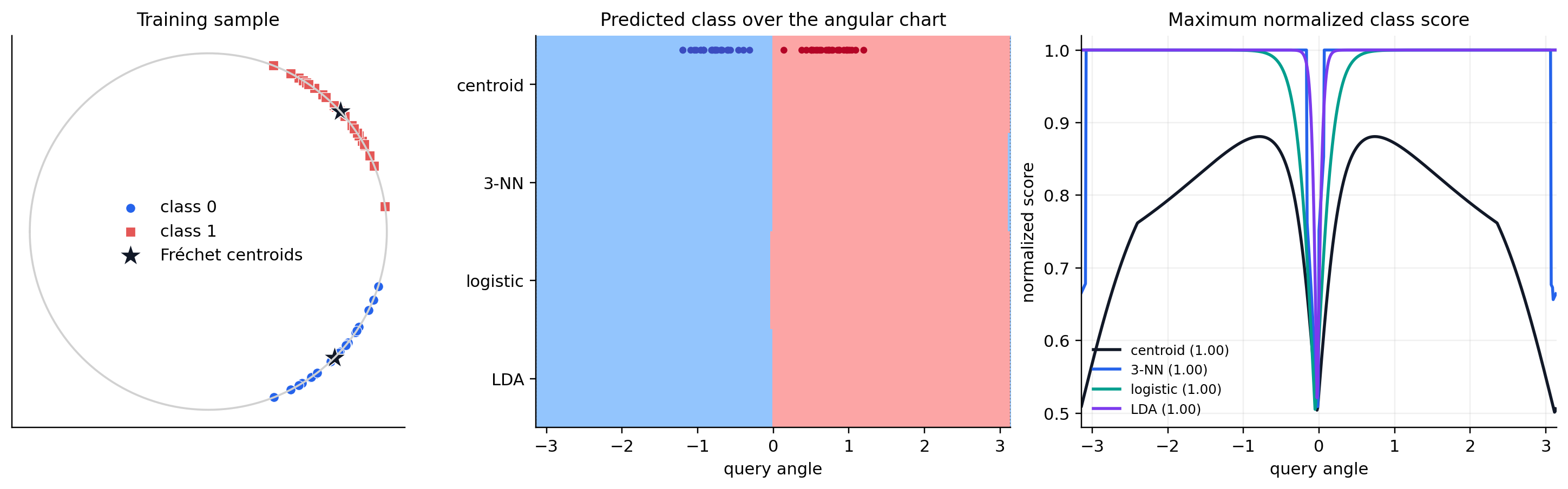
Nearest-centroid prediction is interpretable and stable when classes are unimodal. k-NN adapts to nonlinear class regions but stores the complete training set. Tangent logistic regression and discriminant analysis connect to familiar supervised models, with the important cost that their coordinates are local to one reference point.

References

[BBCJ12]

Alexandre Barachant, Stéphane Bonnet, Marco Congedo, and Christian Jutten. Multiclass brain–computer interface classification by Riemannian geometry. IEEE Transactions on Biomedical Engineering, 59(4):920–928, 2012. doi:10.1109/TBME.2011.2172210.

[Frechet48]

Maurice Fréchet. Les éléments aléatoires de nature quelconque dans un espace distancié. Annales de l'Institut Henri Poincaré, 10(4):215–310, 1948. URL: https://www.numdam.org/item/AIHP_1948__10_4_215_0/.