Adapting Nested Product Data

Scientific observations often mix geometries. A directional measurement may live on a sphere, a phase may be periodic, and an amplitude may be Euclidean. The product metric combines factor metrics by

\[ d_M(x,y)^2=\sum_{r=1}^R d_{M_r}(x_r,y_r)^2. \]

GeoJAX keeps the factor pytree as the point representation. The data adapter validates all leaves against one shared sample axis, which is the same product construction used by manifold optimization [Absil et al., 2008].

from pathlib import Path

import jax
jax.config.update("jax_enable_x64", True)
import jax.numpy as jnp
import matplotlib.pyplot as plt
import numpy as np

from geojax.geometry import Euclidean, Product, Sphere, Torus
from geojax.learning import as_manifold_data, frechet_mean, pairwise_distances

plt.rcParams.update({
    "figure.dpi": 220,
    "savefig.dpi": 320,
    "font.size": 10,
    "axes.titlesize": 11,
    "axes.spines.top": False,
    "axes.spines.right": False,
})

M = Product({
    "direction": Sphere(2),
    "state": (Torus(1), Euclidean(1)),
})

n_samples = 24
angle = jnp.linspace(0.25, 2.15, n_samples)
phase = 0.7 * jnp.sin(1.8 * angle)
amplitude = (1.0 + 0.3 * jnp.cos(angle))[:, None]

# Each leaf arrives in a natural domain representation, not GeoJAX's canonical one.
raw = {
    "direction": angle[:, None],
    "state": (
        jnp.stack([jnp.cos(phase), jnp.sin(phase)], axis=-1)[:, None, :],
        amplitude,
    ),
}
representations = {
    "direction": "hyperspherical",
    "state": ("unit_circle", "canonical"),
}

data = as_manifold_data(M, raw, representation=representations)
print("sample count:", data.n_samples)
print("batch shape:", data.batch_shape)
print("factor tree:", jax.tree_util.tree_structure(data.values))
print("all product points valid:", bool(jnp.all(M.belongs(data.values))))

sample count: 24
batch shape: ()
factor tree: PyTreeDef({'direction': *, 'state': (*, *)})
all product points valid: True

Reuse one validated object

Once adapted, ManifoldData can pass between learning methods without repeating membership checks. The Fréchet mean is computed leafwise through Product geometry while the distance matrix combines the factor contributions.

distances = pairwise_distances(M, data)
mean = frechet_mean(M, data, maxiter=100, tol=1e-9)

mean_direction = np.asarray(mean.point["direction"])
mean_phase = float(mean.point["state"][0][0])
mean_amplitude = float(mean.point["state"][1][0])
print("mean direction:", np.round(mean_direction, 4))
print("mean phase:", f"{mean_phase:.4f}")
print("mean amplitude:", f"{mean_amplitude:.4f}")
print("Fréchet termination:", mean.reason)

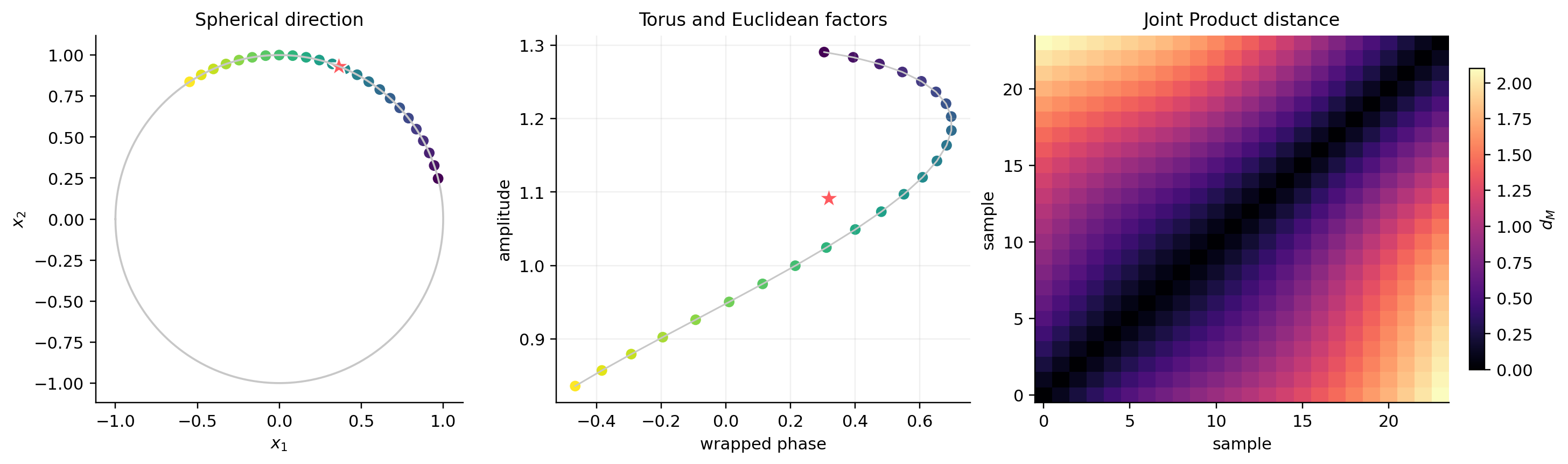
mean direction: [0.3561 0.9344]
mean phase: 0.3278
mean amplitude: 1.0908
Fréchet termination: Last stepsize smaller than options.minstepsize = 1e-10.

Visual report

The panels expose each representation and their joint product distance. The heat map is not any one factor’s distance: it is the metric combination above.

direction = np.asarray(data.values["direction"])
canonical_phase = np.asarray(data.values["state"][0])[:, 0]
canonical_amplitude = np.asarray(data.values["state"][1])[:, 0]

fig, axes = plt.subplots(1, 3, figsize=(13.1, 3.8), constrained_layout=True)
theta = np.linspace(-np.pi, np.pi, 400)
axes[0].plot(np.cos(theta), np.sin(theta), color="0.78", linewidth=1.2)
axes[0].scatter(direction[:, 0], direction[:, 1], c=np.arange(n_samples), cmap="viridis", s=30)
axes[0].scatter(*mean_direction, marker="*", s=180, color="#FF5A5F", edgecolor="white")
axes[0].set(aspect="equal", xlim=(-1.12, 1.12), ylim=(-1.12, 1.12), title="Spherical direction")
axes[0].set_xlabel("$x_1$")
axes[0].set_ylabel("$x_2$")

axes[1].plot(canonical_phase, canonical_amplitude, color="0.78", linewidth=1)
axes[1].scatter(canonical_phase, canonical_amplitude, c=np.arange(n_samples), cmap="viridis", s=30)
axes[1].scatter(mean_phase, mean_amplitude, marker="*", s=180, color="#FF5A5F", edgecolor="white")
axes[1].set(xlabel="wrapped phase", ylabel="amplitude", title="Torus and Euclidean factors")
axes[1].grid(alpha=0.18)

image = axes[2].imshow(np.asarray(distances), cmap="magma", origin="lower", aspect="auto")
axes[2].set(xlabel="sample", ylabel="sample", title="Joint Product distance")
fig.colorbar(image, ax=axes[2], shrink=0.82, label="$d_M$")

output = next(
    path for path in (
        Path("../_static/tutorials/product-adapter.png"),
        Path("docs/_static/tutorials/product-adapter.png"),
        Path("_static/tutorials/product-adapter.png"),
    )
    if path.parent.exists()
)
output.parent.mkdir(parents=True, exist_ok=True)
fig.savefig(output, bbox_inches="tight")
plt.show()

An inconsistent sample count, a different nested structure, or an off-manifold leaf is rejected before pairwise computation begins. Alternate axes are allowed only when sample_axis is supplied explicitly.

References

[AMS08]

P.-A. Absil, Robert Mahony, and Rodolphe Sepulchre. Optimization Algorithms on Matrix Manifolds. Princeton University Press, 2008. doi:10.1515/9781400830244.