svcca

Description

Compute pairwise singular vector CCA (SVCCA) similarities between multiple representations (Raghu et al. 2017). SVCCA first mean-centers and denoises each representation via SVD, retaining components explaining a high fraction of variance at 99% threshold. Then, CCA is applied to the reduced representations, and the similarity is summarized with either Yanai’s GCD (Ramsay, ten Berge, and Styan 1984) or Pillai’s trace (Raghu et al. 2017).

Usage

Python

repsim.svcca(mats, summary_type = None)

R

svcca(mats, summary_type = NULL)

Arguments

Python

• mats: sequence of array-like, length \(M\) List or tuple of M data representations, each of shape (n_samples, n_features_k). All matrices must share the same number of rows for matching samples. Each element can be a NumPy array or any object convertible to one via numpy.asarray.
• summary_type: str, optional Summary statistic for canonical correlations. One of "yanai" and "pillai". Defaults to "yanai".

R

• mats: A list of length M containing data matrices of size (n_samples, n_features_k). All matrices must share the same number of rows for matching samples.
• summary_type: Character scalar indicating the CCA summary statistic. One of "yanai" or "pillai". Defaults to "yanai" if NULL.

Returns

Python

numpy.ndarray

Array of shape (M, M) of SVCCA summary similarities.

R

matrix

An (M, M) symmetric matrix of SVCCA summary similarities.

Examples

Python

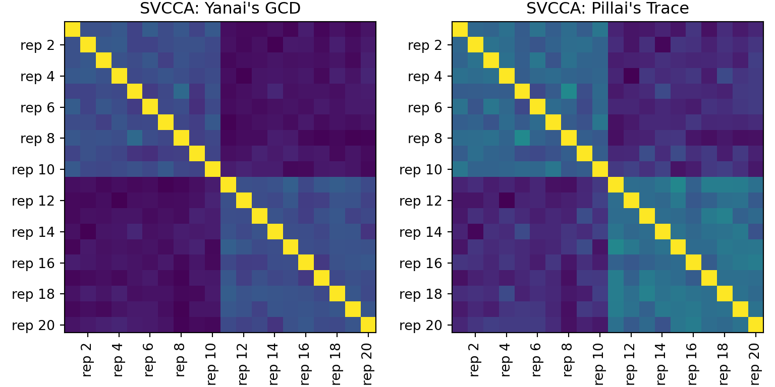
# | cache: true
# load necessary packages
import numpy as np
import pandas as pd
import matplotlib.pyplot as plt
from sklearn.datasets import load_iris
from sklearn.preprocessing import StandardScaler
import repsim

# set a random seed
np.random.seed(1)

# prepare the prototype
iris = load_iris(as_frame=True).frame.iloc[:, :4]
url = "https://vincentarelbundock.github.io/Rdatasets/csv/datasets/USArrests.csv"
usarrests = pd.read_csv(url, index_col=0)

X = StandardScaler().fit_transform(iris.sample(50, random_state=1))
Y = StandardScaler().fit_transform(usarrests)

n, p_X, p_Y = X.shape[0], X.shape[1], Y.shape[1]

# generate 10 of each by perturbation
mats = []
for _ in range(10):
    mats.append(X + np.random.normal(scale=1.0, size=(n, p_X)))
for _ in range(10):
    mats.append(Y + np.random.normal(scale=1.0, size=(n, p_Y)))

# compute similarities
svcca_gcd = repsim.svcca(mats, summary_type="yanai")
svcca_trace = repsim.svcca(mats, summary_type="pillai")

# visualize: two heatmaps side by side
fig, axes = plt.subplots(1, 2, figsize=(8, 4), constrained_layout=True)
titles = ["SVCCA: Yanai's GCD", "SVCCA: Pillai's Trace"]
mats_show = [svcca_gcd, svcca_trace]

labs = [f"rep {i}" for i in range(1, 21)]
even_idx = list(range(1, 20, 2))

for ax, mat, title in zip(axes, mats_show, titles):
    im = ax.imshow(mat, origin="upper")
    ax.set_title(title)
    _ = ax.set_xticks(even_idx)
    _ = ax.set_xticklabels([labs[i] for i in even_idx], rotation=90)
    _ = ax.set_yticks(even_idx)
    _ = ax.set_yticklabels([labs[i] for i in even_idx])

plt.show()

R

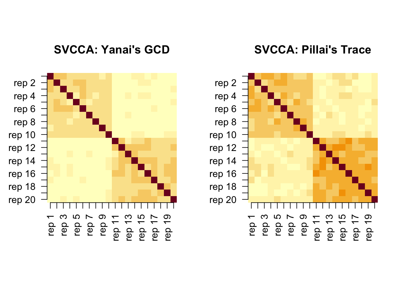
# load necessary packages
library(repsim)

# set a random seed
set.seed(1)

# prepare the prototype
X <- as.matrix(scale(as.matrix(iris[sample(1:150, 50, replace = FALSE), 1:4])))
Y <- as.matrix(scale(as.matrix(USArrests)))
n   <- nrow(X)
p_X <- ncol(X)
p_Y <- ncol(Y)

# generate 10 of each by perturbation
mats <- vector("list", length = 20L)
for (i in 1:10){
  mats[[i]] <- X + matrix(rnorm(n * p_X, sd = 1), nrow = n)
}
for (j in 11:20){
  mats[[j]] <- Y + matrix(rnorm(n * p_Y, sd = 1), nrow = n)
}

# compute similarities
svcca_gcd   <- svcca(mats, summary_type = "yanai")
svcca_trace <- svcca(mats, summary_type = "pillai")

# visualize: two heatmaps side by side
labs <- paste0("rep ", 1:20)
par(pty = "s", mfrow = c(1, 2))

image(svcca_gcd[, 20:1], axes = FALSE, main = "SVCCA: Yanai's GCD")
axis(1, seq(0, 1, length.out = 20), labels = labs, las = 2)
axis(2, at = seq(0, 1, length.out = 20), labels = rev(labs), las = 2)

image(svcca_trace[, 20:1], axes = FALSE, main = "SVCCA: Pillai's Trace")
axis(1, seq(0, 1, length.out = 20), labels = labs, las = 2)
axis(2, at = seq(0, 1, length.out = 20), labels = rev(labs), las = 2)

References

Raghu, Maithra, Justin Gilmer, Jason Yosinski, and Jascha Sohl-Dickstein. 2017. “SVCCA: Singular Vector Canonical Correlation Analysis for Deep Learning Dynamics and Interpretability.” In Proceedings of the 31st International Conference on Neural Information Processing Systems, 6078–87. NIPS’17. Red Hook, NY, USA: Curran Associates Inc.

Ramsay, J. O., Jos ten Berge, and G. P. H. Styan. 1984. “Matrix Correlation.” Psychometrika 49 (3): 403–23.