Transport plans and image interpolation

Images are normalized pixel masses. Choose coordinates explicitly so that comparisons and interpolation use the same geometry. The legacy image interpolation wrapper uses normalized coordinates, increasing rightwards and upwards. This differs from the default pixel-center coordinates of ot_image().

a <- b <- matrix(0, 8, 12)
a[2, 2] <- 2; a[3, 3] <- 1; a[6, 4] <- 3
b[2, 9] <- 1; b[5, 8] <- 3; b[7, 10] <- 2
x <- seq(0, 1, length.out = ncol(a))
y <- seq(1, 0, length.out = nrow(a))
mu <- ot_image(a, x = x, y = y)
nu <- ot_image(b, x = x, y = y)
exact <- ot_distance(mu, nu, method = "exact", return_plan = TRUE)
entropic <- ot_distance(mu, nu, method = "sinkhorn", epsilon = .03,
                        return_plan = TRUE)
ot_inspect(exact)
#> Transport report | finite | unregularized_transport 
#> Producer: ot_distance 
#> Status: SUCCESS ( optimal_pivot_condition )
#>             distance       transport_cost  transport_cost_root 
#>            0.5719694            0.3271490            0.5719694 
#> wasserstein_distance 
#>            0.5719694 
#> Scope: reported stopping criterion only; interpret its reason and available checks
ot_inspect(entropic)
#> Transport report | finite | entropic_transport 
#> Producer: ot_distance 
#> Status: SUCCESS ( marginal_tolerance )
#>              distance        transport_cost   transport_cost_root 
#>             0.5723935             0.3276344             0.5723935 
#> regularized_objective 
#>             0.2501863 
#> Scope: reported stopping criterion only; interpret its reason and available checks

The entropy objective and the unregularized transport cost are separate quantities. The rooted transport component of an entropic plan is not the exact Wasserstein distance.

times <- c(0, .25, .5, .75, 1)
path <- imageinterp(a, b, t = times)
lapply(path[c(1, 3, 5)], ot_inspect)
#> [[1]]
#> Transport report | finite | displacement_interpolation 
#> Producer: imageinterp 
#> Status: SUCCESS ( exact_plan_then_nearest_grid_projection )
#> Scope: exact plan followed by display projection; the displayed image need not be an exact geodesic 
#> 
#> [[2]]
#> Transport report | finite | displacement_interpolation 
#> Producer: imageinterp 
#> Status: SUCCESS ( exact_plan_then_nearest_grid_projection )
#> Scope: exact plan followed by display projection; the displayed image need not be an exact geodesic 
#> 
#> [[3]]
#> Transport report | finite | displacement_interpolation 
#> Producer: imageinterp 
#> Status: SUCCESS ( exact_plan_then_nearest_grid_projection )
#> Scope: exact plan followed by display projection; the displayed image need not be an exact geodesic

For each time, the returned matrix deposits mass at the nearest original grid point. Its unprojected_measure attribute retains the actual push-forward of the optimal plan. The latter follows the exact finite W2 geodesic, up to numerical precision. The displayed matrices generally do not.

mid <- attr(path[[3]], "unprojected_measure")
c(distance_to_midpoint = ot_distance(mu, mid)$wasserstein_distance,
  half_endpoint_distance = exact$wasserstein_distance / 2,
  projection_bound = attr(path[[3]], "diagnostics")$projection_w2_upper_bound)
#>   distance_to_midpoint half_endpoint_distance       projection_bound 
#>             0.28598472             0.28598472             0.06395362
stopifnot(max(abs(vapply(path, sum, numeric(1)) - 1)) < 1e-12)

old <- par(mfrow = c(1, 3), mar = c(1, 1, 2, 1))
for (i in c(1, 3, 5)) {
  image(x, rev(y), t(path[[i]][nrow(a):1, ]),
        axes = FALSE, asp = 1, main = paste("t =", times[i]))
}

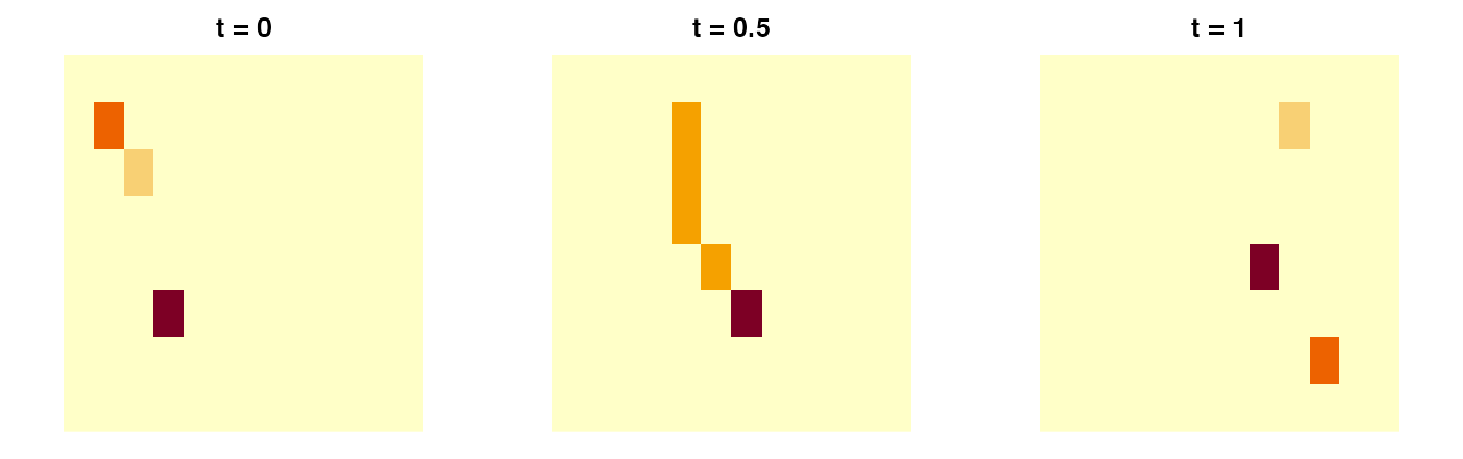
par(old)

The separate replication study verifies all five times, independently reconstructs the transported measures, and quantifies the display error. The images here are deterministic synthetic examples with no data download.