Wasserstein Distance by Inexact Proximal Point Method

Due to high computational cost for linear programming approaches to compute Wasserstein distance, Cuturi (2013) proposed an entropic regularization scheme as an efficient approximation to the original problem. This comes with a regularization parameter $\lambda > 0$ in the term $$\lambda h(\Gamma) = \lambda \sum_{m,n} \Gamma_{m,n} \log (\Gamma_{m,n}).$$ IPOT algorithm is known to be relatively robust to the choice of regularization parameter $\lambda$. Empirical observation says that very small number of inner loop iteration like L=1 is sufficient.

Usage

ipot(X, Y, p = 2, wx = NULL, wy = NULL, lambda = 1, ...)

ipotD(D, p = 2, wx = NULL, wy = NULL, lambda = 1, ...)

Arguments

X

an $(M\times P)$ matrix of row observations.

Y

an $(N\times P)$ matrix of row observations.

p

an exponent for the order of the distance (default: 2).

wx

a length-$M$ marginal density that sums to $1$. If NULL (default), uniform weight is set.

wy

a length-$N$ marginal density that sums to $1$. If NULL (default), uniform weight is set.

lambda

a regularization parameter (default: 0.1).

...

extra parameters including

maxiter: maximum number of iterations (default: 496).
abstol: stopping criterion for iterations (default: 1e-10).
L: small number of inner loop iterations (default: 1).

D

an $(M\times N)$ distance matrix $d(x_m, y_n)$ between two sets of observations.

Value

a named list containing

distance: $\mathcal{W}_p$ distance value
iteration: the number of iterations it took to converge.
plan: an $(M\times N)$ nonnegative matrix for the optimal transport plan.

References

Xie Y, Wang X, Wang R, Zha H (2020). “A fast proximal point method for computing exact wasserstein distance.” In Adams RP, Gogate V (eds.), Proceedings of The 35th Uncertainty in Artificial Intelligence Conference, volume 115 of Proceedings of machine learning research, 433--453.

Examples

# \donttest{
#-------------------------------------------------------------------
#  Wasserstein Distance between Samples from Two Bivariate Normal
#
# * class 1 : samples from Gaussian with mean=(-1, -1)
# * class 2 : samples from Gaussian with mean=(+1, +1)
#-------------------------------------------------------------------
## SMALL EXAMPLE
set.seed(100)
m = 20
n = 30
X = matrix(rnorm(m*2, mean=-1),ncol=2) # m obs. for X
Y = matrix(rnorm(n*2, mean=+1),ncol=2) # n obs. for Y

## COMPARE WITH WASSERSTEIN 
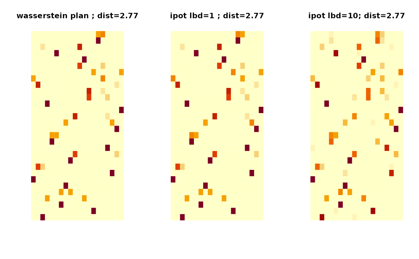
outw = wasserstein(X, Y)
ipt1 = ipot(X, Y, lambda=1)
ipt2 = ipot(X, Y, lambda=10)

## VISUALIZE : SHOW THE PLAN AND DISTANCE
pmw = paste0("wasserstein plan ; dist=",round(outw$distance,2))
pm1 = paste0("ipot lbd=1 ; dist=",round(ipt1$distance,2))
pm2 = paste0("ipot lbd=10; dist=",round(ipt2$distance,2))

opar <- par(no.readonly=TRUE)
par(mfrow=c(1,3))
image(outw$plan, axes=FALSE, main=pmw)
image(ipt1$plan, axes=FALSE, main=pm1)
image(ipt2$plan, axes=FALSE, main=pm2)

par(opar)
# }