Wasserstein Distance via Linear Programming

Given two empirical measures $$\mu = \sum_{m=1}^M \mu_m \delta_{X_m}\quad\textrm{and}\quad \nu = \sum_{n=1}^N \nu_n \delta_{Y_n},$$ the $p$-Wasserstein distance for $p\geq 1$ is posited as the following optimization problem $$ W_p^p(\mu, \nu) = \min_{\pi \in \Pi(\mu, \nu)} \sum_{m=1}^M \sum_{n=1}^N \pi_{mn} \|X_m - Y_n\|^p, $$ where $\Pi(\mu, \nu)$ denotes the set of joint distributions (transport plans) with marginals $\mu$ and $\nu$. This function solves the above problem with linear programming, which is a standard approach for exact computation of the empirical Wasserstein distance. Please see the section for detailed description on the usage of the function.

Usage

wasserstein(X, Y, p = 2, wx = NULL, wy = NULL)

wassersteinD(D, p = 2, wx = NULL, wy = NULL)

Arguments

X: an $(M\times P)$ matrix of row observations.
Y: an $(N\times P)$ matrix of row observations.
p: an exponent for the order of the distance (default: 2).
wx: a length-$M$ marginal density that sums to $1$. If NULL (default), uniform weight is set.
wy: a length-$N$ marginal density that sums to $1$. If NULL (default), uniform weight is set.
D: an $(M\times N)$ distance matrix $d(x_m, y_n)$ between two sets of observations.

Value

a named list containing

distance: $\mathcal{W}_p$ distance value.
plan: an $(M\times N)$ nonnegative matrix for the optimal transport plan.

Using `wasserstein()` function

We assume empirical measures are defined on the Euclidean space $\mathcal{X}=\mathbb{R}^d$, $$\mu = \sum_{m=1}^M \mu_m \delta_{X_m}\quad\textrm{and}\quad \nu = \sum_{n=1}^N \nu_n \delta_{Y_n}$$ and the distance metric used here is standard Euclidean norm $d(x,y) = \|x-y\|$. Here, the marginals $(\mu_1,\mu_2,\ldots,\mu_M)$ and $(\nu_1,\nu_2,\ldots,\nu_N)$ correspond to wx and wy, respectively.

Using `wassersteinD()` function

If other distance measures or underlying spaces are one's interests, we have an option for users to provide a distance matrix D rather than vectors, where $$D := D_{M\times N} = d(X_m, Y_n)$$ for arbitrary distance metrics beyond the $\ell_2$ norm.

References

Peyré G, Cuturi M (2019). “Computational Optimal Transport: With Applications to Data Science.” Foundations and Trends® in Machine Learning, 11(5-6), 355–607. ISSN 1935-8237, 1935-8245, doi:10.1561/2200000073 .

Examples

#-------------------------------------------------------------------
#  Wasserstein Distance between Samples from Two Bivariate Normal
#
# * class 1 : samples from Gaussian with mean=(-1, -1)
# * class 2 : samples from Gaussian with mean=(+1, +1)
#-------------------------------------------------------------------
## SMALL EXAMPLE
m = 20
n = 10
X = matrix(rnorm(m*2, mean=-1),ncol=2) # m obs. for X
Y = matrix(rnorm(n*2, mean=+1),ncol=2) # n obs. for Y

## COMPUTE WITH DIFFERENT ORDERS
out1 = wasserstein(X, Y, p=1)
out2 = wasserstein(X, Y, p=2)
out5 = wasserstein(X, Y, p=5)

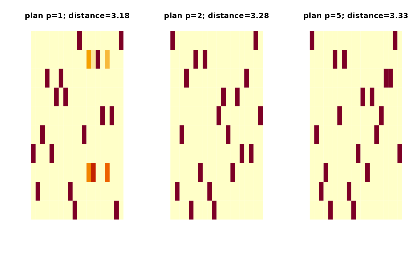
## VISUALIZE : SHOW THE PLAN AND DISTANCE
pm1 = paste0("Order p=1\n distance=",round(out1$distance,2))
pm2 = paste0("Order p=2\n distance=",round(out2$distance,2))
pm5 = paste0("Order p=5\n distance=",round(out5$distance,2))

opar <- par(no.readonly=TRUE)
par(mfrow=c(1,3), pty="s")
image(out1$plan, axes=FALSE, main=pm1)
image(out2$plan, axes=FALSE, main=pm2)
image(out5$plan, axes=FALSE, main=pm5)

par(opar)

if (FALSE) { # \dontrun{
## COMPARE WITH ANALYTIC RESULTS
#  For two Gaussians with same covariance, their 
#  2-Wasserstein distance is known so let's compare !

niter = 1000          # number of iterations
vdist = rep(0,niter)
for (i in 1:niter){
  mm = sample(30:50, 1)
  nn = sample(30:50, 1)
  
  X = matrix(rnorm(mm*2, mean=-1),ncol=2)
  Y = matrix(rnorm(nn*2, mean=+1),ncol=2)
  
  vdist[i] = wasserstein(X, Y, p=2)$distance
  if (i%%10 == 0){
    print(paste0("iteration ",i,"/", niter," complete.")) 
  }
}

# Visualize
opar <- par(no.readonly=TRUE)
hist(vdist, main="Monte Carlo Simulation")
abline(v=sqrt(8), lwd=2, col="red")
par(opar)
} # }