Given \(N\) observations \(X_1, X_2, \ldots, X_N \in \mathcal{M}\),
perform clustering of the data based on the nonlinear mean shift algorithm.
Gaussian kernel is used with the bandwidth \(h\) as of
$$G(x_i, x_j) \propto \exp \left( - \frac{\rho^2 (x_i,x_j)}{h^2} \right)$$
where \(\rho(x,y)\) is geodesic distance between two points \(x,y\in\mathcal{M}\).
Numerically, some of the limiting points that collapse into the same cluster are
not exact. For such purpose, we require maxk parameter to search the
optimal number of clusters based on \(k\)-medoids clustering algorithm
in conjunction with silhouette criterion.
Arguments
- riemobj
a S3
"riemdata"class for \(N\) manifold-valued data.- h
bandwidth parameter. The larger the \(h\) is, the more blurring is applied.
- maxk
maximum number of clusters to determine the optimal number of clusters.
- maxiter
maximum number of iterations to be run.
- eps
tolerance level for stopping criterion.
Value
a named list containing
- distance
an \((N\times N)\) distance between modes corresponding to each data point.
- cluster
a length-\(N\) vector of class labels.
References
Subbarao R, Meer P (2009). “Nonlinear Mean Shift over Riemannian Manifolds.” International Journal of Computer Vision, 84(1), 1–20. ISSN 0920-5691, 1573-1405.
Examples
#-------------------------------------------------------------------
# Example on Sphere : a dataset with three types
#
# class 1 : 10 perturbed data points near (1,0,0) on S^2 in R^3
# class 2 : 10 perturbed data points near (0,1,0) on S^2 in R^3
# class 3 : 10 perturbed data points near (0,0,1) on S^2 in R^3
#-------------------------------------------------------------------
## GENERATE DATA
set.seed(496)
ndata = 10
mydata = list()
for (i in 1:ndata){
tgt = c(1, stats::rnorm(2, sd=0.1))
mydata[[i]] = tgt/sqrt(sum(tgt^2))
}
for (i in (ndata+1):(2*ndata)){
tgt = c(rnorm(1,sd=0.1),1,rnorm(1,sd=0.1))
mydata[[i]] = tgt/sqrt(sum(tgt^2))
}
for (i in ((2*ndata)+1):(3*ndata)){
tgt = c(stats::rnorm(2, sd=0.1), 1)
mydata[[i]] = tgt/sqrt(sum(tgt^2))
}
myriem = wrap.sphere(mydata)
mylabs = rep(c(1,2,3), each=ndata)
## RUN NONLINEAR MEANSHIFT FOR DIFFERENT 'h' VALUES
run1 = riem.nmshift(myriem, maxk=10, h=0.1)
run2 = riem.nmshift(myriem, maxk=10, h=1)
run3 = riem.nmshift(myriem, maxk=10, h=10)
## MDS FOR VISUALIZATION
mds2d = riem.mds(myriem, ndim=2)$embed
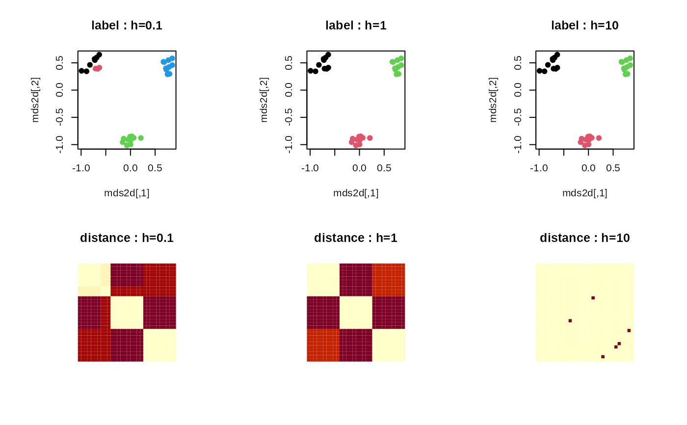
## VISUALIZE
opar <- par(no.readonly=TRUE)
par(mfrow=c(2,3), pty="s")
plot(mds2d, pch=19, main="label : h=0.1", col=run1$cluster)
plot(mds2d, pch=19, main="label : h=1", col=run2$cluster)
plot(mds2d, pch=19, main="label : h=10", col=run3$cluster)
image(run1$distance[,30:1], axes=FALSE, main="distance : h=0.1")
image(run2$distance[,30:1], axes=FALSE, main="distance : h=1")
image(run3$distance[,30:1], axes=FALSE, main="distance : h=10")
 par(opar)