Hierarchical Agglomerative Clustering

Given \(N\) observations \(X_1, X_2, \ldots, X_M \in \mathcal{M}\), perform hierarchical agglomerative clustering with stats::hclust. The supplied manifold distances are treated as dissimilarities.

Usage

riem.hclust(
  riemobj,
  geometry = NULL,
  method = c("single", "complete", "average", "mcquitty", "ward.D", "ward.D2",
    "centroid", "median"),
  members = NULL
)

Arguments

riemobj

a S3 "riemdata" class for \(N\) manifold-valued data.

geometry

A geometry name or saved specification.

method

agglomeration method to be used. This must be one of "single", "complete", "average", "mcquitty", "ward.D", "ward.D2", "centroid" or "median".

members

NULL or a vector whose length equals the number of observations. See hclust for details.

Value

an object of class hclust. See hclust for details.

Details

Ward, centroid and median linkage require care when interpreted as Euclidean sums of squares. In particular, Ward linkage of geodesic distances is not manifold k-means. ward.D is the historical R update and does not implement the Ward criterion implemented by ward.D2. See the stats::hclust documentation for distance powers and member weights.

References

Müllner D (2013). “fastcluster : Fast Hierarchical, Agglomerative Clustering Routines for R and Python.” Journal of Statistical Software, 53(9). ISSN 1548-7660.

Examples

#-------------------------------------------------------------------
#          Example on Sphere : a dataset with three types
#
# class 1 : 10 perturbed data points near (1,0,0) on S^2 in R^3
# class 2 : 10 perturbed data points near (0,1,0) on S^2 in R^3
# class 3 : 10 perturbed data points near (0,0,1) on S^2 in R^3
#-------------------------------------------------------------------
## GENERATE DATA
mydata = list()
for (i in 1:10){
  tgt = c(1, stats::rnorm(2, sd=0.1))
  mydata[[i]] = tgt/sqrt(sum(tgt^2))
}
for (i in 11:20){
  tgt = c(rnorm(1,sd=0.1),1,rnorm(1,sd=0.1))
  mydata[[i]] = tgt/sqrt(sum(tgt^2))
}
for (i in 21:30){
  tgt = c(stats::rnorm(2, sd=0.1), 1)
  mydata[[i]] = tgt/sqrt(sum(tgt^2))
}
myriem = wrap.sphere(mydata)

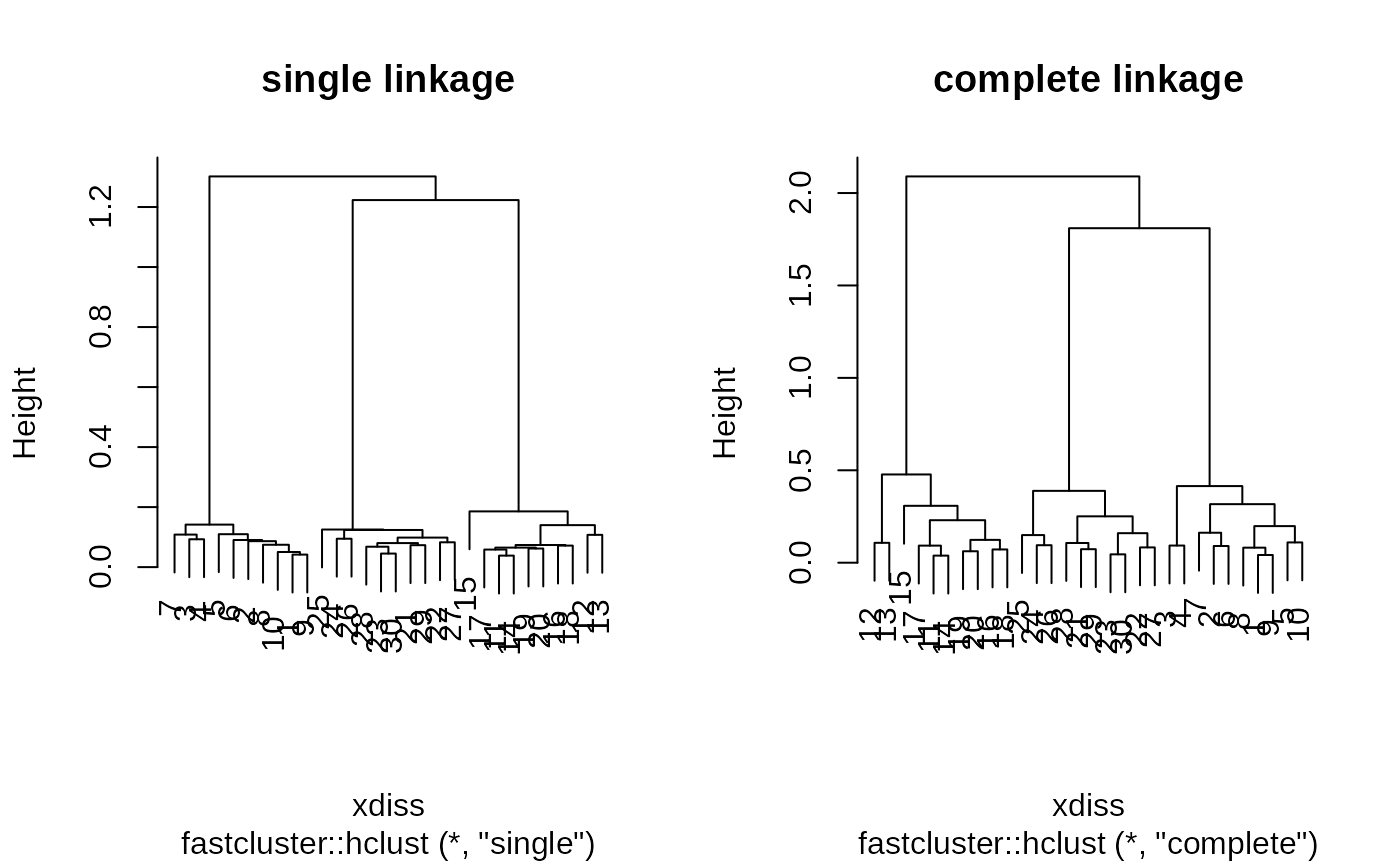
## COMPUTE SINGLE AND COMPLETE LINKAGE
hc.sing <- riem.hclust(myriem, method="single")
hc.comp <- riem.hclust(myriem, method="complete")

## VISUALIZE
opar <- par(no.readonly=TRUE)
par(mfrow=c(1,2))
plot(hc.sing, main="single linkage")
plot(hc.comp, main="complete linkage")

par(opar)