Matrix Angular Central Gaussian Distribution

For Stiefel and Grassmann manifolds $St(r,p)$ and $Gr(r,p)$, the matrix variant of ACG distribution is known as Matrix Angular Central Gaussian (MACG) distribution $MACG_{p,r}(\Sigma)$ with density $$f(X\vert \Sigma) = |\Sigma|^{-r/2} |X^\top \Sigma^{-1} X|^{-p/2}$$ where $\Sigma$ is a $(p\times p)$ symmetric positive-definite matrix. Similar to vector-variate ACG case, we follow a convention that $tr(\Sigma)=p$.

Usage

dmacg(datalist, Sigma)

rmacg(n, r, Sigma)

mle.macg(datalist, ...)

Arguments

datalist

a list of $(p\times r)$ orthonormal matrices.

Sigma

a $(p\times p)$ symmetric positive-definite matrix.

n

the number of samples to be generated.

r

the number of basis.

...

extra parameters for computations, including

maxiter: maximum number of iterations to be run (default:50).
eps: tolerance level for stopping criterion (default: 1e-5).

Value

dmacg gives a vector of evaluated densities given samples. rmacg generates $(p\times r)$ orthonormal matrices wrapped in a list. mle.macg estimates the SPD matrix $\Sigma$.

References

Chikuse Y (1990). “The matrix angular central Gaussian distribution.” Journal of Multivariate Analysis, 33(2), 265--274. ISSN 0047259X.

Mardia KV, Jupp PE (eds.) (1999). Directional Statistics, Wiley Series in Probability and Statistics. John Wiley \& Sons, Inc., Hoboken, NJ, USA. ISBN 978-0-470-31697-9 978-0-471-95333-3.

Kent JT, Ganeiber AM, Mardia KV (2013). "A new method to simulate the Bingham and related distributions in directional data analysis with applications." arXiv:1310.8110.

Examples

# -------------------------------------------------------------------
#          Example with Matrix Angular Central Gaussian Distribution
#
# Given a fixed Sigma, generate samples and estimate Sigma via ML.
# -------------------------------------------------------------------
## GENERATE AND MLE in St(2,5)/Gr(2,5)
#  Generate data
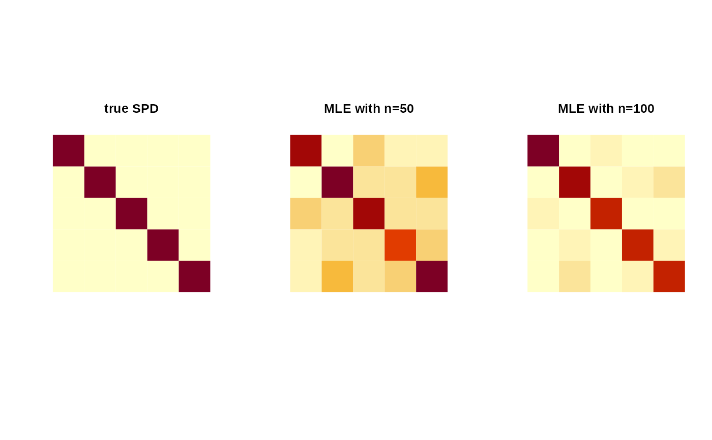
Strue = diag(5)                  # true SPD matrix
sam1  = rmacg(n=50,  r=2, Strue) # random samples
sam2  = rmacg(n=100, r=2, Strue) # random samples

#  MLE
Smle1 = mle.macg(sam1)
Smle2 = mle.macg(sam2)

#  Visualize
opar <- par(no.readonly=TRUE)
par(mfrow=c(1,3), pty="s")
image(Strue[,5:1], axes=FALSE, main="true SPD")
image(Smle1[,5:1], axes=FALSE, main="MLE with n=50")
image(Smle2[,5:1], axes=FALSE, main="MLE with n=100")

par(opar)