t-distributed Stochastic Neighbor Embedding

\(t\)-distributed Stochastic Neighbor Embedding (t-SNE) is a variant of Stochastic Neighbor Embedding (SNE) that mimicks patterns of probability distributinos over pairs of high-dimensional objects on low-dimesional target embedding space by minimizing Kullback-Leibler divergence. While conventional SNE uses gaussian distributions to measure similarity, t-SNE, as its name suggests, exploits a heavy-tailed Student t-distribution.

do.tsne(
  X,
  ndim = 2,
  perplexity = 30,
  eta = 0.05,
  maxiter = 2000,
  jitter = 0.3,
  jitterdecay = 0.99,
  momentum = 0.5,
  pca = TRUE,
  pcascale = FALSE,
  symmetric = FALSE,
  BHuse = TRUE,
  BHtheta = 0.25
)

Arguments

X

an \((n\times p)\) matrix or data frame whose rows are observations and columns represent independent variables.

ndim

an integer-valued target dimension.

perplexity

desired level of perplexity; ranging [5,50].

eta

learning parameter.

maxiter

maximum number of iterations.

jitter

level of white noise added at the beginning.

jitterdecay

decay parameter in (0,1). The closer to 0, the faster artificial noise decays.

momentum

level of acceleration in learning.

pca

whether to use PCA as preliminary step; TRUE for using it, FALSE otherwise.

pcascale

a logical; FALSE for using Covariance, TRUE for using Correlation matrix. See also do.pca for more details.

symmetric

a logical; FALSE to solve it naively, and TRUE to adopt symmetrization scheme.

BHuse

a logical; TRUE to use Barnes-Hut approximation. See Rtsne for more details.

BHtheta

speed-accuracy tradeoff. If set as 0.0, it reduces to exact t-SNE.

Value

a named Rdimtools S3 object containing

Y

an \((n\times ndim)\) matrix whose rows are embedded observations.

algorithm

name of the algorithm.

References

van der Maaten L, Hinton G (2008). “Visualizing Data Using T-SNE.” The Journal of Machine Learning Research, 9(2579-2605), 85.

See also

do.sne

Author

Kisung You

Examples

# \donttest{
## load iris data
data(iris)
set.seed(100)
subid = sample(1:150,50)
X     = as.matrix(iris[subid,1:4])
lab   = as.factor(iris[subid,5])

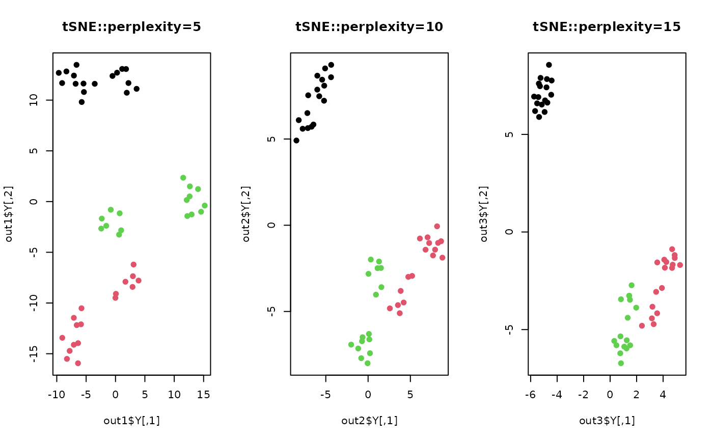
## compare different perplexity
out1 <- do.tsne(X, ndim=2, perplexity=5)
out2 <- do.tsne(X, ndim=2, perplexity=10)
out3 <- do.tsne(X, ndim=2, perplexity=15)

## Visualize three different projections
opar <- par(no.readonly=TRUE)
par(mfrow=c(1,3))
plot(out1$Y, pch=19, col=lab, main="tSNE::perplexity=5")
plot(out2$Y, pch=19, col=lab, main="tSNE::perplexity=10")
plot(out3$Y, pch=19, col=lab, main="tSNE::perplexity=15")

par(opar)
# }