Wasserstein Distance Estimation with Boostrapping

This function computes the \(\mathcal{W}_p\) distance between two empirical measures using bootstrap in order to quantify the uncertainty of the estimation.

Usage

wassboot(X, Y, p = 2, B = 500, wx = NULL, wy = NULL)

Arguments

X

an \((M\times P)\) matrix of row observations.

Y

an \((N\times P)\) matrix of row observations.

p

an exponent for the order of the distance (default: 2).

B

number of bootstrap samples (default: 500).

wx

a length-\(M\) marginal density that sums to \(1\). If NULL (default), uniform weight is set.

wy

a length-\(N\) marginal density that sums to \(1\). If NULL (default), uniform weight is set.

Value

a named list containing

distance

\(\mathcal{W}_p\) distance value.

boot_samples

a length-\(B\) vector of bootstrap samples.

Examples

# \donttest{
#-------------------------------------------------------------------
#  Boostrapping Wasserstein Distance between Two Bivariate Normals
#
# * class 1 : samples from Gaussian with mean=(-5, 0)
# * class 2 : samples from Gaussian with mean=(+5, 0)
#-------------------------------------------------------------------
## SMALL EXAMPLE
m = round(runif(1, min=50, max=100))
n = round(runif(1, min=50, max=100))
X = matrix(rnorm(m*2), ncol=2) # m obs. for X
Y = matrix(rnorm(n*2), ncol=2) # n obs. for Y

X[,1] = X[,1] - 5
Y[,1] = Y[,1] + 5

## COMPUTE THE BOOTSTRAP SAMPLES
boots = wassboot(X, Y, B=1000)

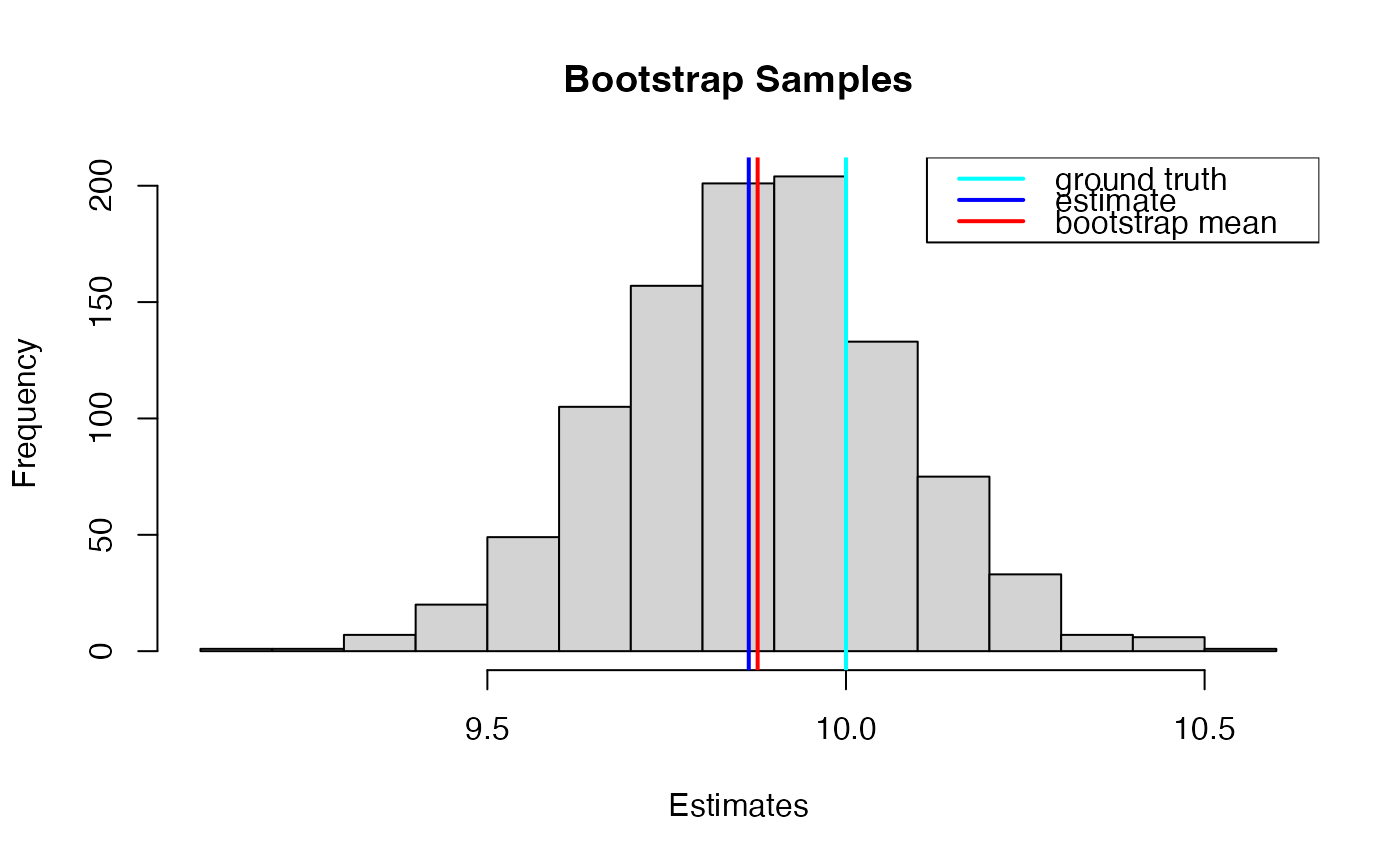
## VISUALIZE
opar <- par(no.readonly=TRUE)
hist(boots$boot_samples, xlab="Estimates", main="Bootstrap Samples")
abline(v=boots$distance, lwd=2, col="blue")
abline(v=mean(boots$boot_samples), lwd=2, col="red")
abline(v=10, col="cyan", lwd=2)
legend("topright", c("ground truth","estimate","bootstrap mean"), 
        col=c("cyan","blue","red"), lwd=2)

par(opar)
# }