Sliced Wasserstein Distance

Sliced Wasserstein (SW) Distance (Rabin et al. 2012) is a popular alternative to the standard Wasserstein distance due to its computational efficiency on top of nice theoretical properties. For the \(d\)-dimensional probability measures \(\mu\) and \(\nu\), the SW distance is defined as $$\mathcal{SW}_p (\mu, \nu) = \left( \int_{\mathbf{S}^{d-1}} \mathcal{W}_p^p ( \langle \theta, \mu\rangle, \langle \theta, \nu \rangle d\lambda (\theta) \right)^{1/p},$$ where \(\mathbf{S}^{d-1}\) is the \((d-1)\)-dimensional unit hypersphere and \(\lambda\) is the uniform distribution on \(\mathbf{S}^{d-1}\). Practically, it is computed via Monte Carlo integration.

Usage

swdist(X, Y, p = 2, ...)

Arguments

X

an \((M\times P)\) matrix of row observations.

Y

an \((N\times P)\) matrix of row observations.

p

an exponent for the order of the distance (default: 2).

...

extra parameters including

nproj

the number of Monte Carlo samples for SW computation (default: 496).

Value

a named list containing

distance

\(\mathcal{SW}_p\) distance value.

projdist

a length-niter vector of projected univariate distances.

References

Rabin J, Peyré G, Delon J, Bernot M (2012). “Wasserstein Barycenter and Its Application to Texture Mixing.” In Bruckstein AM, ter Haar Romeny BM, Bronstein AM, Bronstein MM (eds.), Scale Space and Variational Methods in Computer Vision, volume 6667, 435--446. Springer Berlin Heidelberg, Berlin, Heidelberg.

Examples

# \donttest{
#-------------------------------------------------------------------
#  Sliced-Wasserstein Distance between Two Bivariate Normal
#
# * class 1 : samples from Gaussian with mean=(-1, -1)
# * class 2 : samples from Gaussian with mean=(+1, +1)
#-------------------------------------------------------------------
# SMALL EXAMPLE
set.seed(100)
m = 20
n = 30
X = matrix(rnorm(m*2, mean=-1),ncol=2) # m obs. for X
Y = matrix(rnorm(n*2, mean=+1),ncol=2) # n obs. for Y

# COMPUTE THE SLICED-WASSERSTEIN DISTANCE
outsw <- swdist(X, Y, nproj=100)

# VISUALIZE
# prepare ingredients for plotting
plot_x = 1:1000
plot_y = base::cumsum(outsw$projdist)/plot_x

# draw
opar <- par(no.readonly=TRUE)
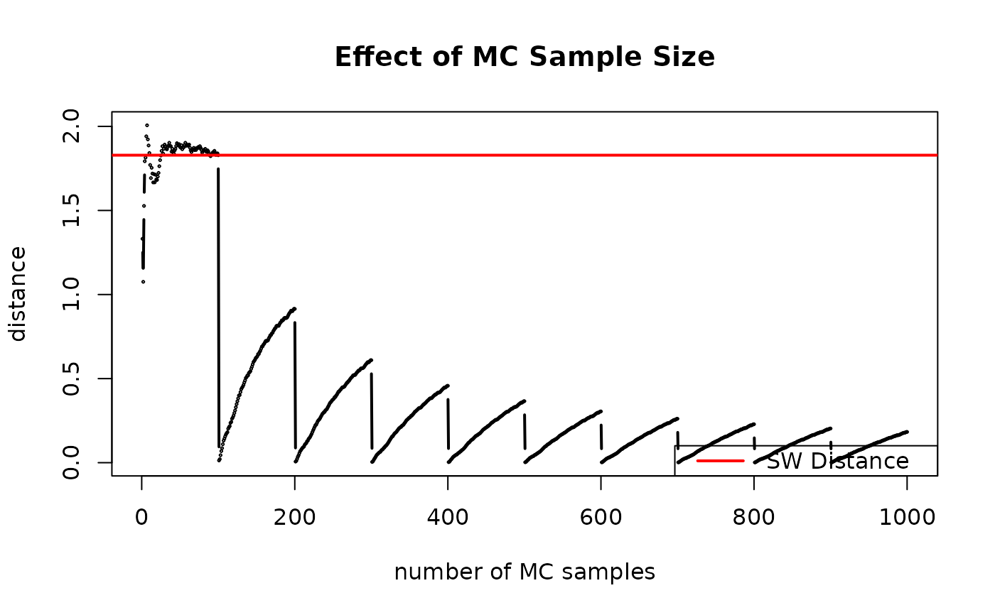
plot(plot_x, plot_y, type="b", cex=0.1, lwd=2,
     xlab="number of MC samples", ylab="distance",
     main="Effect of MC Sample Size")
abline(h=outsw$distance, col="red", lwd=2)
legend("bottomright", legend="SW Distance", 
       col="red", lwd=2)

par(opar)
# }