Free-Support Barycenter by Riemannian gradient descent

For a collection of empirical measures \(\lbrace \mu_k\rbrace_{k=1}^K\), the free-support barycenter of order 2 is computed using the Riemannian gradient descent algorithm. The algorithm is based on the formal Riemannian geometric view of the 2-Wasserstein space according to Otto (2001) .

Usage

rbaryGD(atoms, marginals = NULL, weights = NULL, num_support = 100, ...)

Arguments

atoms

a length-\(K\) list where each element is an \((N_k \times P)\) matrix of atoms.

marginals

marginal distributions for empirical measures; if NULL (default), uniform weights are set for all measures. Otherwise, it should be a length-\(K\) list where each element is a length-\(N_i\) vector of nonnegative weights that sum to 1.

weights

weights for each individual measure; if NULL (default), each measure is considered equally. Otherwise, it should be a length-\(K\) vector.

num_support

the number of support points \(M\) for the barycenter (default: 100).

...

extra parameters including

abstol

stopping criterion for iterations (default: 1e-6).

maxiter

maximum number of iterations (default: 10).

Value

a list with three elements:

support

an \((M \times P)\) matrix of barycenter support points.

weight

a length-\(M\) vector of barycenter weights with all entries being \(1/M\).

history

a vector of cost values at each iteration.

References

Otto F (2001). “The Geometry of Dissipative Evolution Equations: The Porous Medium Equation.” Communications in Partial Differential Equations, 26(1-2), 101–174. ISSN 0360-5302, 1532-4133, doi:10.1081/PDE-100002243 .

Examples

# \donttest{
#-------------------------------------------------------------------
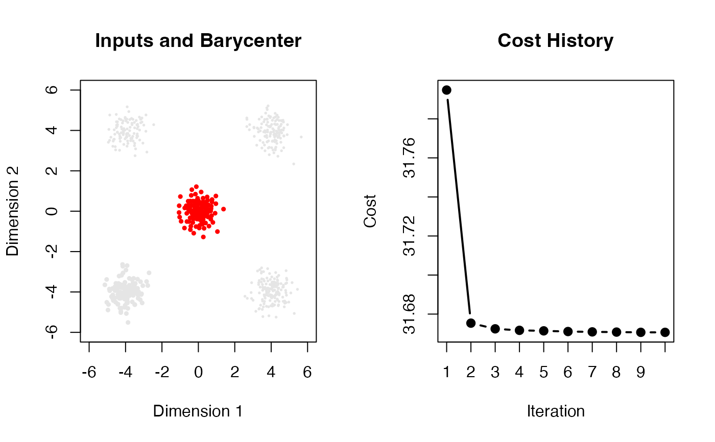
#     Free-Support Wasserstein Barycenter of Four Gaussians
#
# * class 1 : samples from Gaussian with mean=(-4, -4)
# * class 2 : samples from Gaussian with mean=(+4, +4)
# * class 3 : samples from Gaussian with mean=(+4, -4)
# * class 4 : samples from Gaussian with mean=(-4, +4)
#
#  All measures have uniform weights.
#-------------------------------------------------------------------
## GENERATE DATA
#  Empirical Measures
set.seed(100)
unif4 = round(runif(4, 100, 200))
dat1 = matrix(rnorm(unif4[1]*2, mean=-4, sd=0.5),ncol=2)
dat2 = matrix(rnorm(unif4[2]*2, mean=+4, sd=0.5),ncol=2) 
dat3 = cbind(rnorm(unif4[3], mean=+4, sd=0.5), rnorm(unif4[3], mean=-4, sd=0.5))
dat4 = cbind(rnorm(unif4[4], mean=-4, sd=0.5), rnorm(unif4[4], mean=+4, sd=0.5))

myatoms = list()
myatoms[[1]] = dat1
myatoms[[2]] = dat2
myatoms[[3]] = dat3
myatoms[[4]] = dat4

## COMPUTE
fsbary = rbaryGD(myatoms)

## VISUALIZE
#  aligned with CRAN convention
opar <- par(no.readonly=TRUE, mfrow=c(1,2))

#  plot the input measures and the barycenter
plot(myatoms[[1]], col="gray90", pch=19, cex=0.5, xlim=c(-6,6), ylim=c(-6,6), 
     main="Inputs and Barycenter", xlab="Dimension 1", ylab="Dimension 2")
points(myatoms[[2]], col="gray90", pch=19, cex=0.25)
points(myatoms[[3]], col="gray90", pch=19, cex=0.25)
points(myatoms[[4]], col="gray90", pch=19, cex=0.25)
points(fsbary$support, col="red", cex=0.5, pch=19)

#  plot the cost history with only integer ticks
plot(seq_along(fsbary$history), fsbary$history, type="b", lwd=2, pch=19,
     main="Cost History", xlab="Iteration", ylab="Cost", xaxt='n')
axis(1, at=seq_along(fsbary$history))

par(opar)
# }