Interpolation between Histograms

Given two histograms represented as "histogram" S3 objects with identical breaks, compute interpolated histograms along the 2-Wasserstein geodesic connecting them. In 1D, this is achieved by linear interpolation of quantile functions (displacement interpolation).

Usage

histinterp(hist1, hist2, t = 0.5, L = 2000L)

Arguments

hist1

a histogram ("histogram" object).

hist2

another histogram with the same breaks as hist1.

t

a scalar or numeric vector in \([0,1]\) specifying interpolation times. t = 0 returns hist1, t = 1 returns hist2.

L

number of quantile levels used to approximate the geodesic (default: 2000). Larger L gives a more accurate approximation at increased computational cost.

Value

If length(t) == 1, a single "histogram" object representing the interpolated distribution at time t. If length(t) > 1, a length-length(t) list of "histogram" objects.

Examples

# \donttest{
#----------------------------------------------------------------------
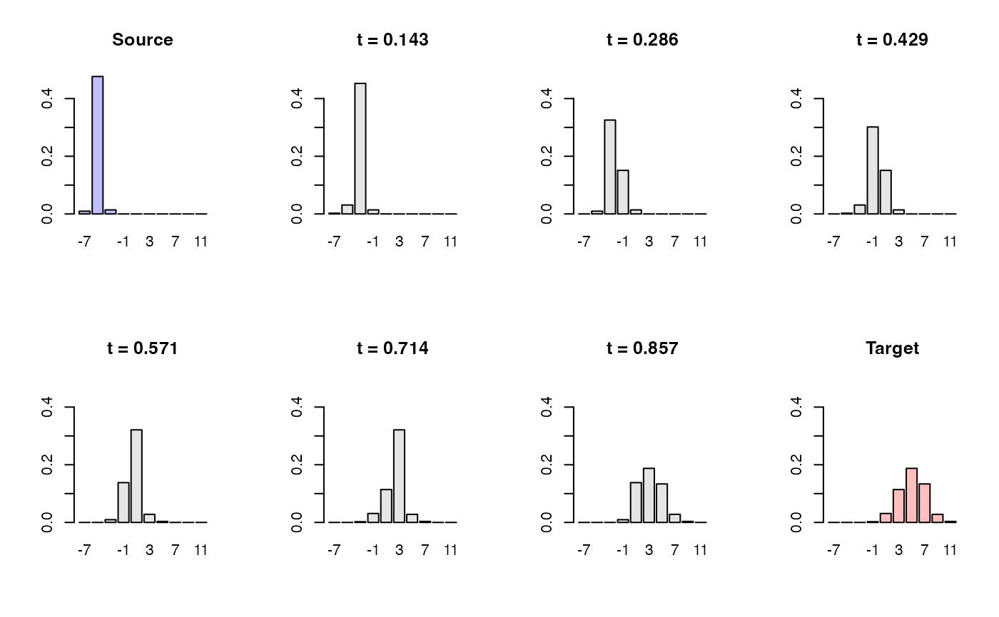
#                      Interpolating Two Gaussians
#
# The source histogram is created from N(-5,1/4).
# The target histogram is created from N(+5,4)
#----------------------------------------------------------------------
# SETTING
set.seed(123)
x_source = rnorm(1000, mean=-5, sd=1/2)
x_target = rnorm(1000, mean=+5, sd=2)

# BUILD HISTOGRAMS WITH COMMON BREAKS
bk = seq(from=-8, to=12, by=2)
h1 = hist(x_source, breaks=bk, plot=FALSE)
h2 = hist(x_target, breaks=bk, plot=FALSE)

# INTERPOLATE WITH 5 GRID POINTS
h_path <- histinterp(h1, h2, t = seq(0, 1, length.out = 8))

# VISUALIZE
y_slim <- c(0, max(h1$density, h2$density)) # shared y-limit
xt     <- round(h1$mids, 1) # x-ticks

opar <- par(no.readonly = TRUE)
par(mfrow = c(2,4), pty = "s")
for (i in 1:8){
  if (i < 2){
    barplot(h_path[[i]]$density,  names.arg=xt, ylim=y_slim,
            main="Source", col=rgb(0,0,1,1/4))
  } else if (i > 7){
    barplot(h_path[[i]]$density,  names.arg=xt, ylim=y_slim,
            main="Target", col=rgb(1,0,0,1/4))
  } else {
    barplot(h_path[[i]]$density,  names.arg=xt, ylim=y_slim, 
            col="gray90", main=sprintf("t = %.3f", (i-1)/7))
  }
}

par(opar)
# }