Spectral Clustering by Ng, Jordan, and Weiss (2002)

The version of Ng, Jordan, and Weiss first constructs the affinity matrix $$A_{ij} = \exp(-d(x_i, d_j)^2 / \sigma^2)$$ where \(\sigma\) is a common bandwidth parameter and performs k-means (or possibly, GMM) clustering on the row-space of eigenvectors for the symmetric graph laplacian matrix $$L=D^{-1/2}(D-A)D^{-1/2}$$.

scNJW(data, k = 2, sigma = 1, ...)

Arguments

data	an \((n\times p)\) matrix of row-stacked observations or S3 dist object of \(n\) observations.
k	the number of clusters (default: 2).
sigma	bandwidth parameter (default: 1).
...	extra parameters including algclust method to perform clustering on embedded data; either "kmeans" (default) or "GMM". maxiter the maximum number of iterations (default: 10).

Value

a named list of S3 class T4cluster containing

cluster

a length-\(n\) vector of class labels (from \(1:k\)).

eigval

eigenvalues of the graph laplacian's spectral decomposition.

embeds

an \((n\times k)\) low-dimensional embedding.

algorithm

name of the algorithm.

References

Ng AY, Jordan MI, Weiss Y (2002). “On Spectral Clustering: Analysis and an Algorithm.” In Dietterich TG, Becker S, Ghahramani Z (eds.), Advances in Neural Information Processing Systems 14, 849--856. MIT Press.

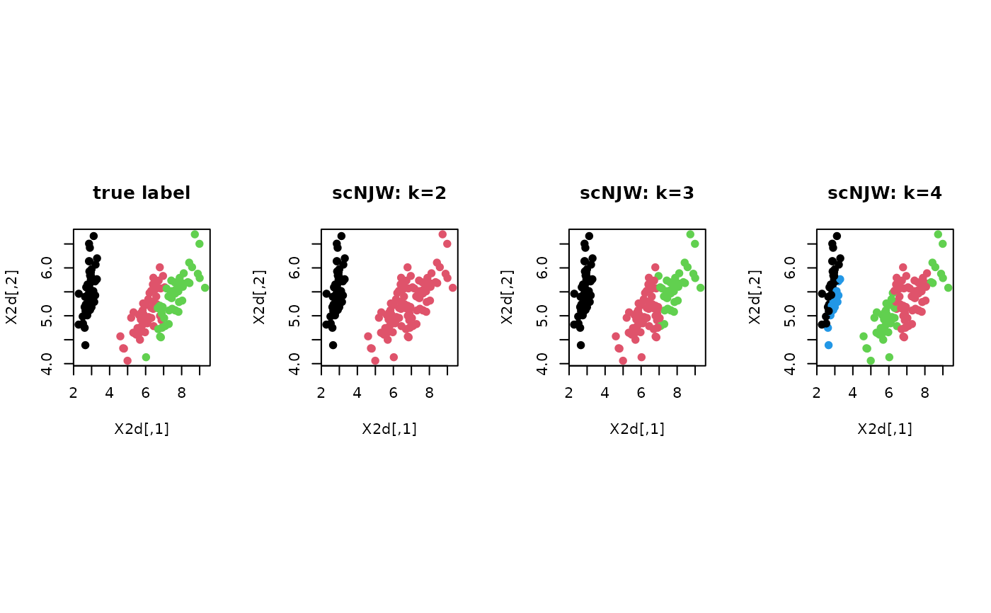
Examples

# -------------------------------------------------------------
#            clustering with 'iris' dataset
# -------------------------------------------------------------
## PREPARE
data(iris)
X   = as.matrix(iris[,1:4])
lab = as.integer(as.factor(iris[,5]))

## EMBEDDING WITH PCA
X2d = Rdimtools::do.pca(X, ndim=2)$Y

## CLUSTERING WITH DIFFERENT K VALUES
cl2 = scNJW(X, k=2)$cluster
cl3 = scNJW(X, k=3)$cluster
cl4 = scNJW(X, k=4)$cluster

## VISUALIZATION
opar <- par(no.readonly=TRUE)
par(mfrow=c(1,4), pty="s")
plot(X2d, col=lab, pch=19, main="true label")
plot(X2d, col=cl2, pch=19, main="scNJW: k=2")
plot(X2d, col=cl3, pch=19, main="scNJW: k=3")
plot(X2d, col=cl4, pch=19, main="scNJW: k=4")
par(opar)