Geodesic Spherical K-Means

Geodesic spherical \(k\)-means algorithm is an counterpart of the spherical \(k\)-means algorithm by replacing the cosine similarity with the squared geodesic distance, which is the great-circle distance under the intrinsic geometry regime on the unit hypersphere. If the data is not normalized, it performs the normalization and proceeds thereafter.

gskmeans(data, k = 2, ...)

Arguments

data	an \((n\times p)\) matrix of row-stacked observations. If not row-stochastic, each row is normalized to be unit norm.
k	the number of clusters (default: 2).
...	extra parameters including init initialization method; either "kmeans" or "gmm" (default: "kmeans"). maxiter the maximum number of iterations (default: 10). abstol stopping criterion to stop the algorithm (default: \(10^{-8}\)). verbose a logical; TRUE to show iteration history or FALSE to quiet.

Value

a named list of S3 class T4cluster containing

cluster

a length-\(n\) vector of class labels (from \(1:k\)).

cost

a value of the cost function.

means

an \((k\times p)\) matrix where each row is a unit-norm class mean.

algorithm

name of the algorithm.

Examples

# \donttest{
# -------------------------------------------------------------
#            clustering with 'household' dataset
# -------------------------------------------------------------
## PREPARE
data(household, package="T4cluster")
X   = household$data
lab = as.integer(household$gender)

## EXECUTE GSKMEANS WITH VARYING K's
vec.rand = rep(0, 9)
for (i in 1:9){
  clust_i = gskmeans(X, k=(i+1))$cluster
  vec.rand[i] = compare.rand(clust_i, lab)
}

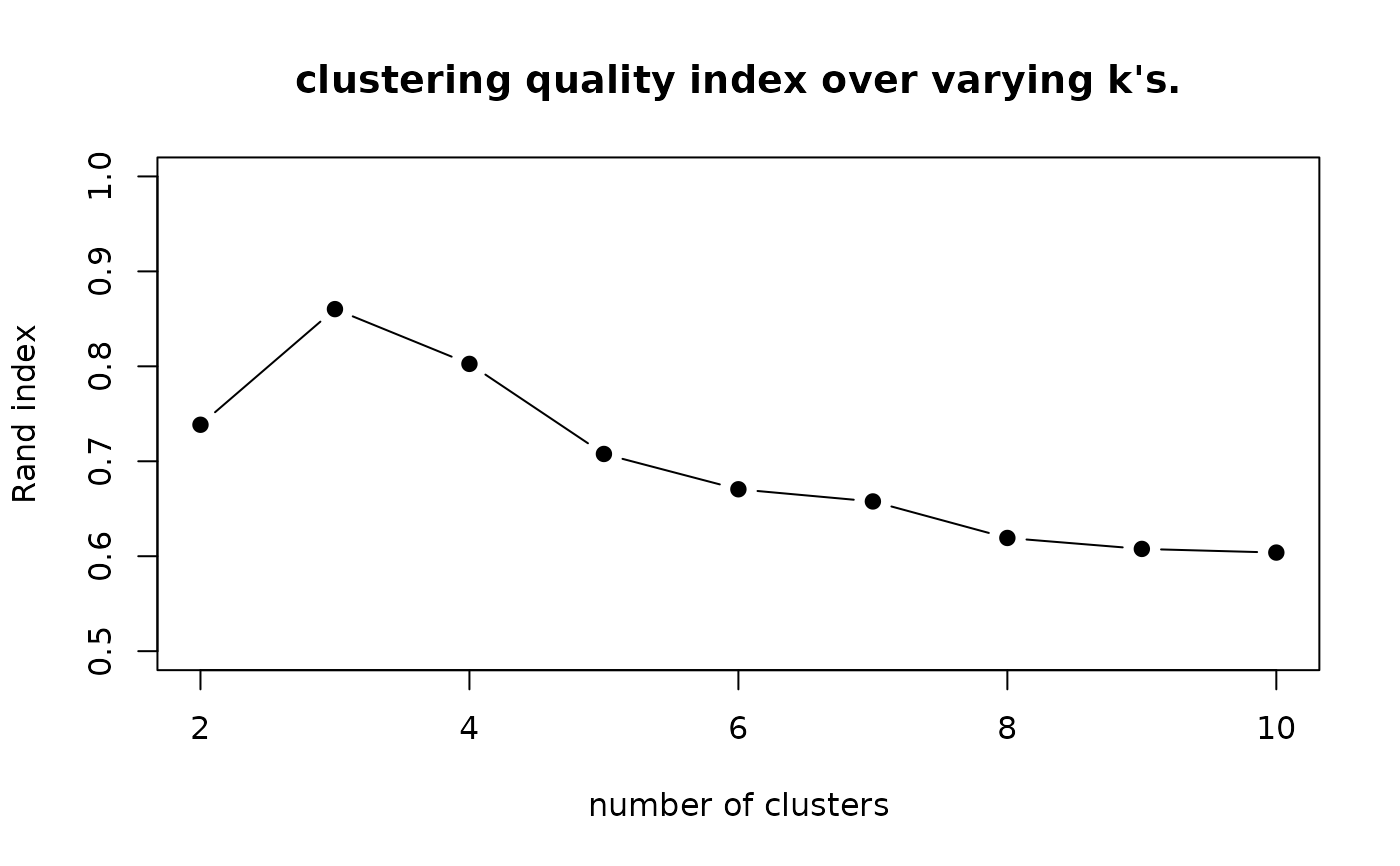
## VISUALIZE THE RAND INDEX
opar <- par(no.readonly=TRUE)
plot(2:10, vec.rand, type="b", pch=19, ylim=c(0.5, 1),
     ylab="Rand index",xlab="number of clusters",
     main="clustering quality index over varying k's.")
par(opar)
# }