Diffusion Maps — do.dm • Rdimtools

do.dm discovers low-dimensional manifold structure embedded in high-dimensional data space using Diffusion Maps (DM). It exploits diffusion process and distances in data space to find equivalent representations in low-dimensional space.

do.dm(
  X,
  ndim = 2,
  preprocess = c("null", "center", "scale", "cscale", "decorrelate", "whiten"),
  bandwidth = 1,
  timescale = 1,
  multiscale = FALSE
)

Arguments

X: an \((n\times p)\) matrix or data frame whose rows are observations and columns represent independent variables.
ndim: an integer-valued target dimension.
preprocess: an additional option for preprocessing the data. Default is "null". See also aux.preprocess for more details.
bandwidth: a scaling parameter for diffusion kernel. Default is 1 and should be a nonnegative real number.
timescale: a target scale whose value represents behavior of heat kernels at time t. Default is 1 and should be a positive real number.
multiscale: logical; FALSE is to use the fixed timescale value, TRUE to ignore the given value.

Value

a named list containing

Y: an \((n\times ndim)\) matrix whose rows are embedded observations.
trfinfo: a list containing information for out-of-sample prediction.
eigvals: a vector of eigenvalues for Markov transition matrix.

References

Nadler B, Lafon S, Coifman RR, Kevrekidis IG (2005). “Diffusion Maps, Spectral Clustering and Eigenfunctions of Fokker-Planck Operators.” In Proceedings of the 18th International Conference on Neural Information Processing Systems, NIPS'05, 955--962.

Coifman RR, Lafon S (2006). “Diffusion Maps.” Applied and Computational Harmonic Analysis, 21(1), 5--30.

Author

Kisung You

Examples

# \donttest{
## load iris data
data(iris)
set.seed(100)
subid = sample(1:150,50)
X     = as.matrix(iris[subid,1:4])
label = as.factor(iris[subid,5])

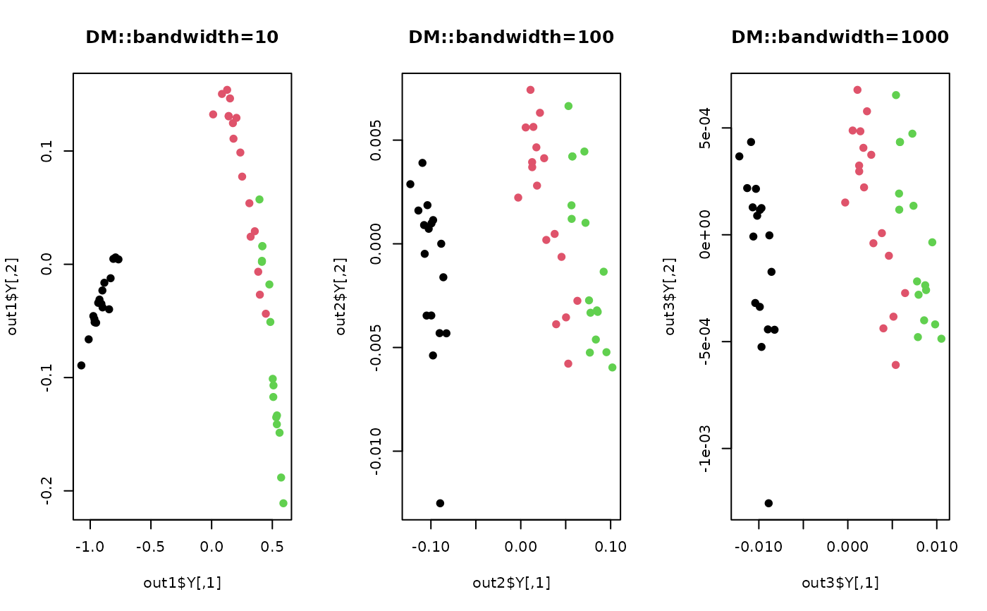
## compare different bandwidths
out1 <- do.dm(X,bandwidth=10)
out2 <- do.dm(X,bandwidth=100)
out3 <- do.dm(X,bandwidth=1000)

## visualize
opar <- par(no.readonly=TRUE)
par(mfrow=c(1,3))
plot(out1$Y, pch=19, col=label, main="DM::bandwidth=10")
plot(out2$Y, pch=19, col=label, main="DM::bandwidth=100")
plot(out3$Y, pch=19, col=label, main="DM::bandwidth=1000")

par(opar)
# }